Note
This page was generated from a Jupyter Notebook. Download the notebook (.ipynb)
[1]:
# Skipped in CI: Colab/bootstrap dependency install cell.
Spectrogram: Normalization and Cleaning
![]()
This tutorial demonstrates two groups of spectrogram post-processing tools available in gwexpy:
API |
Purpose |
|---|---|
|
Convert raw power to SNR or relative units |
|
Remove glitches, trends, and persistent lines |
Prerequisites: Spectrogram Basics
[2]:
import warnings

warnings.filterwarnings("ignore", category=UserWarning)
warnings.filterwarnings("ignore", category=DeprecationWarning)

import matplotlib.pyplot as plt
import numpy as np

from gwexpy.timeseries import TimeSeries

plt.rcParams["figure.figsize"] = (12, 4)
1. Synthetic Data
We build a 2-minute strain time series containing:
Stationary Gaussian noise with a slowly drifting amplitude (non-stationarity)
Persistent narrowband line at 60 Hz (power-line coupling)
Transient glitches at 15 s, 45 s, and 90 s
[3]:
# ── Reproducible seed ────────────────────────────────────────────────────────
rng = np.random.default_rng(42)

DURATION  = 120    # seconds
FS        = 512    # Hz
FFTLEN    = 4.0    # s
STRIDE    = 2.0    # s

t = np.arange(0, DURATION, 1 / FS)

# Base: flat noise (simulate whitened strain)
base_noise = rng.normal(0, 1.0, len(t))

# Add persistent narrowband line at 60 Hz (power line)
line60 = 3.0 * np.sin(2 * np.pi * 60 * t)

# Add slowly drifting broadband noise floor (non-stationary trend)
trend = 1.0 + 0.5 * np.sin(2 * np.pi * t / DURATION)

# Add a few transient glitches (excess-power bursts)
glitch_times = [15.0, 45.0, 90.0]
glitch_signal = np.zeros_like(t)
for gt in glitch_times:
    idx = int(gt * FS)
    width = int(0.05 * FS)
    glitch_signal[idx : idx + width] += rng.normal(0, 8.0, width)

strain = (base_noise * trend) + line60 + glitch_signal

ts = TimeSeries(strain, dt=1.0 / FS, name="STRAIN", unit="strain")
spec = ts.spectrogram2(FFTLEN, overlap=FFTLEN / 2)
print("Spectrogram shape (time × freq):", spec.shape)
print("Time bins:", spec.shape[0], " | Freq bins:", spec.shape[1])
Spectrogram shape (time × freq): (60, 1025)
Time bins: 60  | Freq bins: 1025
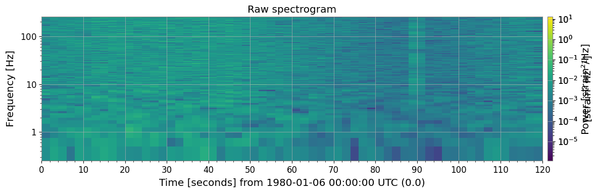
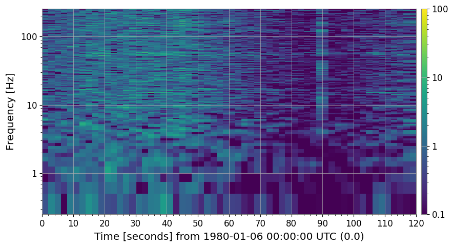
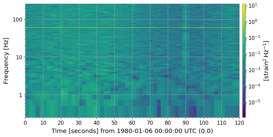
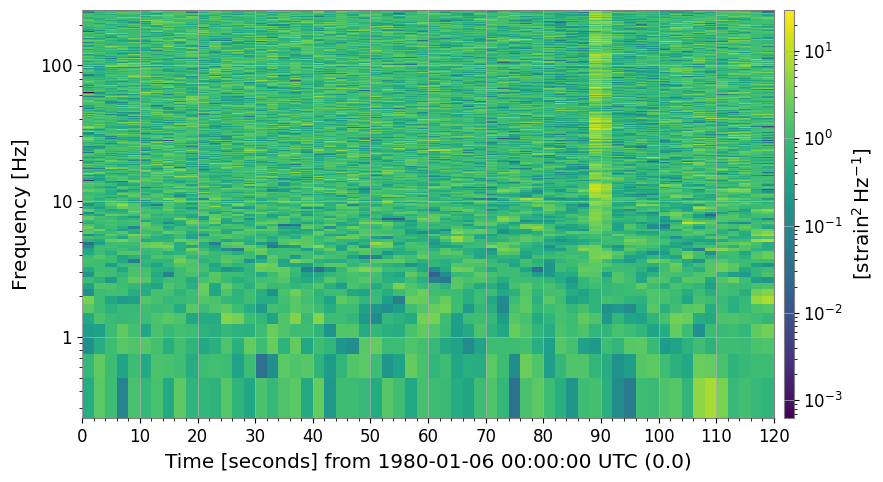
2. Baseline Spectrogram
The raw spectrogram already shows glitches (bright vertical stripes), the 60 Hz line (bright horizontal stripe), and the time-varying noise floor.
[4]:
import warnings

with warnings.catch_warnings():
    warnings.simplefilter('ignore')

    _plt5 = spec.plot(norm="log", figsize=(12, 4))
    ax = _plt5.gca()
    ax.set_title("Raw spectrogram")
    _plt5.colorbar(label="Power [strain²/Hz]")
    with warnings.catch_warnings():
        warnings.filterwarnings("ignore", message="This figure includes Axes that are not compatible with tight_layout")
        plt.tight_layout()
    plt.show()
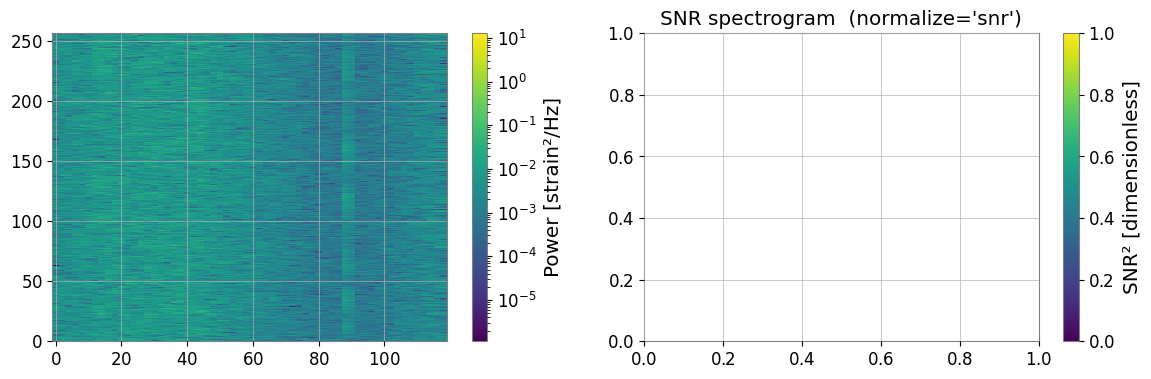
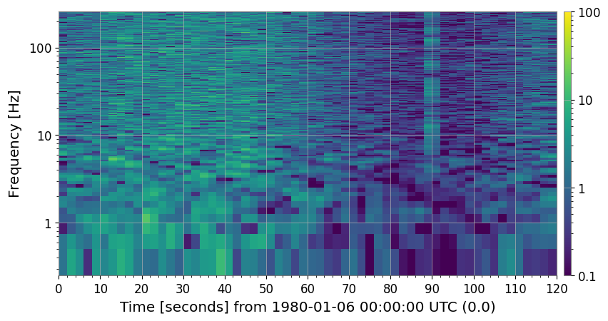
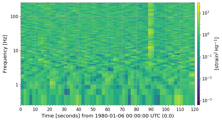
3. Normalization
3a. SNR Spectrogram (method='snr')
[5]:
import warnings

with warnings.catch_warnings():
    warnings.simplefilter('ignore')

    # ── SNR normalization ─────────────────────────────────────────────────────────
    # Each time slice is divided by the median PSD along the time axis.
    # Result: dimensionless SNR² (≈ 1 for stationary background).
    spec_snr = spec.normalize(method="snr")

    fig, axes = plt.subplots(1, 2, figsize=(14, 4))
    _pc0 = axes[0].pcolormesh(spec.times.value, spec.frequencies.value, spec.value.T, norm=__import__("matplotlib.colors", fromlist=["LogNorm"]).LogNorm(), cmap="viridis", shading="auto")
    fig.colorbar(_pc0, ax=axes[0], label="Power [strain²/Hz]")

    spec_snr.plot(ax=axes[1], norm="log", vmin=0.1, vmax=100)
    axes[1].set_title("SNR spectrogram  (normalize='snr')")
    fig.colorbar(next((c for c in axes[1].get_children() if hasattr(c, "get_clim")), None) or __import__("matplotlib.cm", fromlist=["ScalarMappable"]).ScalarMappable(), ax=axes[1], label="SNR² [dimensionless]")

    with warnings.catch_warnings():
        warnings.filterwarnings("ignore", message="This figure includes Axes that are not compatible with tight_layout")
        plt.tight_layout()
    plt.show()
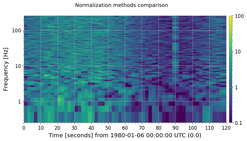
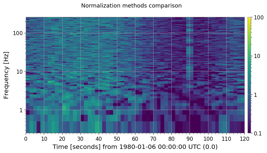
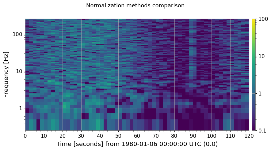
3b. Other Normalization Methods
|
Denominator |
|---|---|
|
Median PSD per frequency bin (identical to |
|
Mean PSD per frequency bin |
|
Nth-percentile PSD (controlled by |
[6]:
import warnings

with warnings.catch_warnings():
    warnings.simplefilter('ignore')

    # ── Compare normalization methods ─────────────────────────────────────────────
    methods = ["median", "mean", "percentile"]
    fig, axes = plt.subplots(1, 3, figsize=(18, 4))
    for ax, m in zip(axes, methods):
        kw = {"percentile": 75.0} if m == "percentile" else {}
        spec_n = spec.normalize(method=m, **kw)
        spec_n.plot(ax=ax, norm="log", vmin=0.1, vmax=100)
        label = "percentile=75" if m == "percentile" else ""
        ax.set_title(f"method='{m}' {label}")
        fig.colorbar(next((c for c in ax.get_children() if hasattr(c, "get_clim")), None), ax=ax, label="SNR² []")
        plt.suptitle("Normalization methods comparison", fontsize=13)
    with warnings.catch_warnings():
        warnings.filterwarnings("ignore", message="This figure includes Axes that are not compatible with tight_layout")
        plt.tight_layout()
    plt.show()
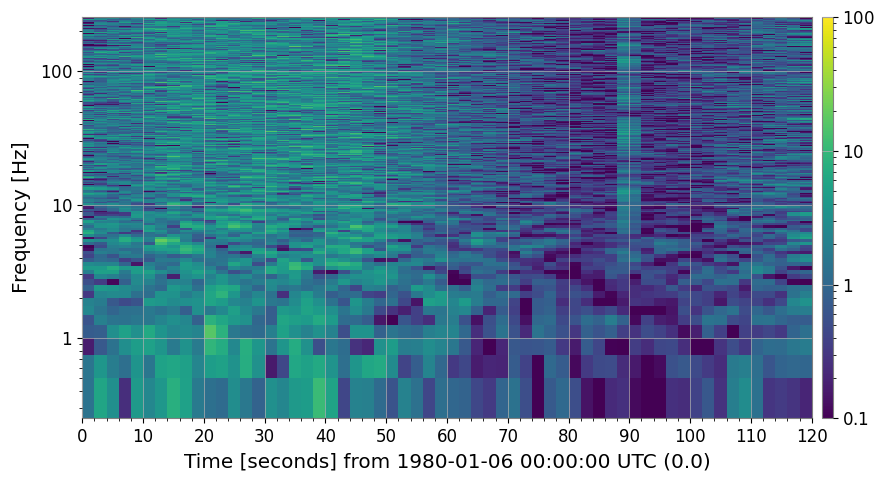
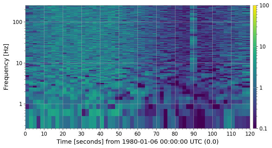
3c. Reference Normalization (method='reference')
Supply your own reference spectrum — useful when you want to compare against a specific quiet period or an independently measured noise floor.
[7]:
import warnings

with warnings.catch_warnings():
    warnings.simplefilter('ignore')

    # ── Reference normalization ───────────────────────────────────────────────────
    # Use the first 30 s as a quiet reference segment.
    quiet_ts = ts.crop(0, 30)
    ref_spec = quiet_ts.spectrogram2(FFTLEN, overlap=FFTLEN / 2)
    reference_psd = np.median(ref_spec.value, axis=0)   # median over the 30-s window

    spec_ref = spec.normalize(method="reference", reference=reference_psd)

    fig, ax = plt.subplots(figsize=(12, 4))
    spec_ref.plot(ax=ax, norm="log", vmin=0.1, vmax=100)
    ax.set_title("Reference-normalized spectrogram (30-s quiet baseline)")
    fig.colorbar(next((c for c in ax.get_children() if hasattr(c, "get_clim")), None), ax=ax, label="SNR² []")
    with warnings.catch_warnings():
        warnings.filterwarnings("ignore", message="This figure includes Axes that are not compatible with tight_layout")
        plt.tight_layout()
    plt.show()
4. Cleaning
4a. Threshold Cleaning (method='threshold')
Pixels that exceed median + threshold × MAD (per frequency bin) are flagged as outliers and replaced. Replacement strategy is controlled by fill= ('median', 'nan', 'zero', or 'interpolate').
This removes short-duration glitches that appear as bright vertical streaks.
[8]:
import warnings

with warnings.catch_warnings():
    warnings.simplefilter('ignore')

    # ── threshold cleaning ────────────────────────────────────────────────────────
    # Pixels exceeding  median + threshold × MAD  are replaced.
    spec_thr, mask = spec_snr.clean(method="threshold", threshold=5.0, return_mask=True)

    print(f"Flagged pixels: {mask.sum()} / {mask.size}"
    f"  ({100 * mask.mean():.2f} %)")

    fig, axes = plt.subplots(1, 2, figsize=(14, 4))
    spec_snr.plot(ax=axes[0], norm="log", vmin=0.1, vmax=100)
    axes[0].set_title("SNR spectrogram (before threshold clean)")
    fig.colorbar(next((c for c in axes[0].get_children() if hasattr(c, "get_clim")), None) or __import__("matplotlib.cm", fromlist=["ScalarMappable"]).ScalarMappable(), ax=axes[0], label="SNR²")

    spec_thr.plot(ax=axes[1], norm="log", vmin=0.1, vmax=100)
    axes[1].set_title("After threshold clean  (threshold=5 MAD)")
    fig.colorbar(next((c for c in axes[1].get_children() if hasattr(c, "get_clim")), None) or __import__("matplotlib.cm", fromlist=["ScalarMappable"]).ScalarMappable(), ax=axes[1], label="SNR²")

    with warnings.catch_warnings():
        warnings.filterwarnings("ignore", message="This figure includes Axes that are not compatible with tight_layout")
        plt.tight_layout()
    plt.show()
Flagged pixels: 2096 / 61500 (3.41 %)
4b. Rolling-Median Detrending (method='rolling_median')
[9]:
import warnings

with warnings.catch_warnings():
    warnings.simplefilter('ignore')

    # ── rolling-median cleaning ───────────────────────────────────────────────────
    # Divide by a rolling median along the time axis to remove slow trends.
    spec_roll = spec.clean(method="rolling_median", window_size=10)

    fig, axes = plt.subplots(1, 2, figsize=(14, 4))
    spec.plot(ax=axes[0], norm="log")
    axes[0].set_title("Raw spectrogram")
    fig.colorbar(next((c for c in axes[0].get_children() if hasattr(c, "get_clim")), None) or __import__("matplotlib.cm", fromlist=["ScalarMappable"]).ScalarMappable(), ax=axes[0], label="Power")

    spec_roll.plot(ax=axes[1], norm="log")
    axes[1].set_title("After rolling-median detrend  (window=10 bins)")
    fig.colorbar(next((c for c in axes[1].get_children() if hasattr(c, "get_clim")), None) or __import__("matplotlib.cm", fromlist=["ScalarMappable"]).ScalarMappable(), ax=axes[1], label="Normalised power []")

    with warnings.catch_warnings():
        warnings.filterwarnings("ignore", message="This figure includes Axes that are not compatible with tight_layout")
        plt.tight_layout()
    plt.show()
4c. Persistent Line Removal (method='line_removal')
amplitude_threshold × global_median for more than persistence_threshold fraction of time bins.[10]:
import warnings

# ── line-removal cleaning ─────────────────────────────────────────────────────
# Detect persistent narrowband lines and replace with column median.
spec_noline, line_indices = spec_snr.clean(
    method="line_removal",
    persistence_threshold=0.8,
    amplitude_threshold=3.0,
    return_mask=True,
)

# line_indices is a bool mask here; retrieve actual frequency values
freq_axis = spec.frequencies.value
if hasattr(line_indices, "sum"):   # ndarray mask
    flagged_freqs = freq_axis[np.any(line_indices, axis=0)]
else:
    flagged_freqs = freq_axis[line_indices]
print("Detected line frequencies [Hz]:", np.round(flagged_freqs, 1))

fig, axes = plt.subplots(1, 2, figsize=(14, 4))
spec_snr.plot(ax=axes[0], norm="log", vmin=0.1, vmax=100)
axes[0].set_title("SNR spectrogram (with 60 Hz power line)")
fig.colorbar(
    next((c for c in axes[0].get_children() if hasattr(c, "get_clim")), None)
    or __import__("matplotlib.cm", fromlist=["ScalarMappable"]).ScalarMappable(),
    ax=axes[0],
    label="SNR²",
)

spec_noline.plot(ax=axes[1], norm="log", vmin=0.1, vmax=100)
axes[1].set_title("After line-removal clean")
fig.colorbar(
    next((c for c in axes[1].get_children() if hasattr(c, "get_clim")), None)
    or __import__("matplotlib.cm", fromlist=["ScalarMappable"]).ScalarMappable(),
    ax=axes[1],
    label="SNR²",
)

with warnings.catch_warnings():
    warnings.filterwarnings(
        "ignore",
        message="This figure includes Axes that are not compatible with tight_layout",
    )
    plt.tight_layout()
plt.show()
Detected line frequencies [Hz]: []


4d. Full Cleaning Pipeline (method='combined')
[11]:
import warnings

with warnings.catch_warnings():
    warnings.simplefilter('ignore')

    # ── combined pipeline ─────────────────────────────────────────────────────────
    # threshold → rolling_median → line_removal in one call.
    spec_clean = spec.clean(
    method="combined",
    threshold=5.0,
    window_size=10,
    persistence_threshold=0.8,
    amplitude_threshold=3.0,
    )

    fig, axes = plt.subplots(1, 2, figsize=(14, 4))
    spec.plot(ax=axes[0], norm="log")
    axes[0].set_title("Raw spectrogram")
    fig.colorbar(next((c for c in axes[0].get_children() if hasattr(c, "get_clim")), None) or __import__("matplotlib.cm", fromlist=["ScalarMappable"]).ScalarMappable(), ax=axes[0], label="Power")

    spec_clean.plot(ax=axes[1], norm="log")
    axes[1].set_title("Fully cleaned spectrogram  (method='combined')")
    fig.colorbar(next((c for c in axes[1].get_children() if hasattr(c, "get_clim")), None) or __import__("matplotlib.cm", fromlist=["ScalarMappable"]).ScalarMappable(), ax=axes[1], label="Normalised power []")

    with warnings.catch_warnings():
        warnings.filterwarnings("ignore", message="This figure includes Axes that are not compatible with tight_layout")
        plt.tight_layout()
    plt.show()

5. Summary
All methods and their purposes:
[12]:
print("=" * 62)
print(f"{'Method':<22} {'Description':<38}")
print("-" * 62)
rows = [
    ("normalize('snr')",       "÷ median PSD  →  SNR² map"),
    ("normalize('median')",    "÷ median PSD  (alias for snr)"),
    ("normalize('mean')",      "÷ mean PSD"),
    ("normalize('percentile')","÷ Nth-percentile PSD"),
    ("normalize('reference')", "÷ user-supplied reference spectrum"),
    ("clean('threshold')",     "Replace MAD-outlier pixels"),
    ("clean('rolling_median')","Divide by rolling-median trend"),
    ("clean('line_removal')",  "Remove persistent narrowband lines"),
    ("clean('combined')",      "threshold → rolling_median → line_removal"),
]
for m, d in rows:
    print(f"  {m:<20} {d}")
print("=" * 62)
==============================================================
Method                 Description
--------------------------------------------------------------
  normalize('snr')     ÷ median PSD  →  SNR² map
  normalize('median')  ÷ median PSD  (alias for snr)
  normalize('mean')    ÷ mean PSD
  normalize('percentile') ÷ Nth-percentile PSD
  normalize('reference') ÷ user-supplied reference spectrum
  clean('threshold')   Replace MAD-outlier pixels
  clean('rolling_median') Divide by rolling-median trend
  clean('line_removal') Remove persistent narrowband lines
  clean('combined')    threshold → rolling_median → line_removal
==============================================================