Note

This page was generated from a Jupyter Notebook. Download the notebook (.ipynb)

# Skipped in CI: Colab/bootstrap dependency install cell.

Glitch Analysis: Q-Transform and Omega-Scan

Glitches are short-duration, non-Gaussian noise transients that contaminate gravitational-wave data. The Q-transform (or Omega scan) is the standard time-frequency representation used to characterise and classify glitches at all major detector sites.

The Q-transform tiles the time-frequency plane with constant-Q (constant bandwidth-to-frequency ratio) windows and measures the normalised energy in each tile. A glitch appears as a cluster of tiles with anomalously high SNR.

What this tutorial covers:

1. Injecting synthetic glitches into a noise background

2. Computing the Q-transform with q_scan() and QTiling

3. Visualising the time-frequency map (Omega scan)

4. Extracting peak SNR, time, and frequency from QGram

5. Characterising glitch morphology (duration, bandwidth, Q)

Related tutorials:

• advanced_peak_detection.ipynb — spectral line detection

• advanced_peak_tracking.ipynb — tracking lines over time

• case_bruco_advanced.ipynb — coherence-based noise coupling

Setup

import warnings

warnings.filterwarnings("ignore", category=UserWarning)
warnings.filterwarnings("ignore", category=DeprecationWarning)

import matplotlib.pyplot as plt
import numpy as _np
import numpy as np
from scipy.stats import kstest as _kstest
from scipy.stats import rayleigh as _rayleigh

from gwexpy.signal.qtransform import q_scan
from gwexpy.timeseries import TimeSeries


def rayleigh_test(data):
    """KS test of data against Rayleigh distribution."""
    data = _np.asarray(data, dtype=float)
    scale = _np.sqrt(_np.mean(data**2) / 2)
    return _kstest(data, _rayleigh(scale=scale).cdf)

1. Synthetic Data with Injected Glitches

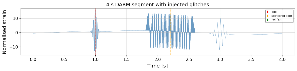
We create a 4 s segment of KAGRA-like DARM noise with three injected glitches representative of common morphologies seen in practice:

Glitch	Morphology	Typical origin
Blip	Short broadband burst	Unknown / scattered light
Scattered light	Arch-shaped frequency sweep	Mirror motion + scattering
Koi fish	Low-frequency with harmonic	Suspension resonance

fs   = 4096.0    # sample rate [Hz]
T    = 4.0       # segment duration [s]
N    = int(T * fs)
t    = np.arange(N) / fs
t0   = 1_300_000_000
rng  = np.random.default_rng(7)

# --- Gaussian noise coloured to LIGO-like O3 sensitivity ---
freqs_n = np.fft.rfftfreq(N, 1.0 / fs)[1:]
# Simplified ASD: f^{-2} below 30 Hz, flat above (units: normalised)
asd = np.where(freqs_n < 30, (30.0 / freqs_n)**2, 1.0)
noise_fft = asd * np.exp(1j * rng.uniform(0, 2*np.pi, size=len(freqs_n)))
noise_fft = np.concatenate([[0.0], noise_fft])
noise = np.fft.irfft(noise_fft, n=N)
noise /= noise.std()   # normalise to unit RMS

# --- Glitch 1: Blip at t=1.0 s, ~100 Hz, Q~8 ---
t_blip = 1.0
f_blip, Q_blip = 100.0, 8.0
tau_blip = Q_blip / (np.pi * f_blip)
envelope_blip = np.exp(-0.5 * ((t - t_blip) / tau_blip)**2)
glitch_blip = 15.0 * envelope_blip * np.sin(2*np.pi*f_blip*(t - t_blip))

# --- Glitch 2: Scattered-light arch at t=2.0–2.5 s ---
# Frequency sweeps as f(t) = f0 * |sin(pi*t/P)|  (mirror pendulum)
t_sl = np.linspace(1.8, 2.6, 500)
f_sl = 50.0 * np.abs(np.sin(np.pi * (t_sl - 1.8) / 0.8))
phi_sl = 2*np.pi * np.cumsum(f_sl) / fs * (t_sl[1] - t_sl[0]) * fs
glitch_sl = np.zeros(N)
idx_sl = ((t_sl - t[0]) * fs).astype(int)
idx_sl = idx_sl[(idx_sl >= 0) & (idx_sl < N)]
glitch_sl[idx_sl[:len(phi_sl[:len(idx_sl)])]] = 12.0 * np.sin(phi_sl[:len(idx_sl)])

# --- Glitch 3: Koi-fish (low-freq + harmonics) at t=3.0 s ---
t_koi = 3.0
f_koi, tau_koi = 20.0, 0.08
env_koi = np.exp(-((t - t_koi) / tau_koi)**2)
glitch_koi = (8.0 * env_koi * np.sin(2*np.pi*f_koi*t) +
              4.0 * env_koi * np.sin(2*np.pi*2*f_koi*t) +
              2.0 * env_koi * np.sin(2*np.pi*3*f_koi*t))

signal = noise + glitch_blip + glitch_sl + glitch_koi
ts = TimeSeries(signal, t0=t0, sample_rate=fs, name="K1:LSC-DARM_OUT_DQ")

fig, ax = plt.subplots(figsize=(12, 3))
ax.plot(t, signal, lw=0.5, color="steelblue", alpha=0.8)
ax.axvline(t_blip, color="red",   ls="--", lw=0.8, label="Blip")
ax.axvline(2.2,    color="orange", ls="--", lw=0.8, label="Scattered light")
ax.axvline(t_koi,  color="green",  ls="--", lw=0.8, label="Koi fish")
ax.set_xlabel("Time [s]")
ax.set_ylabel("Normalised strain")
ax.set_title("4 s DARM segment with injected glitches")
ax.legend(fontsize=8)
plt.tight_layout()
plt.show()

2. Q-Transform (Omega Scan)

q_scan() searches over a range of Q values and returns the tile with the highest normalised energy together with the full QGram object for plotting.

Key parameters:

• qrange — range of Q values to search (default: 4–64)

• frange — frequency range in Hz

• mismatch — fractional tile overlap (smaller = finer grid, slower)

# Whiten the data first (Q-transform assumes white noise for SNR normalisation)
ts_white = ts.whiten(fftlength=1.0, overlap=0.5)

# Run Q-scan over the full segment
qgram, far = q_scan(
    ts_white,
    qrange   = (4, 64),
    frange   = (10, 1200),
    mismatch = 0.2,
)

print("Q-scan result:")
print(f"  Peak SNR      : {qgram.peak['energy']:.1f}")
print(f"  Peak time     : t0 + {qgram.peak['time'] - t0:.3f} s")
print(f"  Peak frequency: {qgram.peak['frequency']:.1f} Hz")
print(f"  Peak Q        : {qgram.peak.get('q', 'N/A')}")
print(f"  Estimated FAR : {far:.2e} Hz")

Q-scan result:
  Peak SNR      : 4565141.5
  Peak time     : t0 + 1.000 s
  Peak frequency: 97.8 Hz
  Peak Q        : N/A
  Estimated FAR : 0.00e+00 Hz

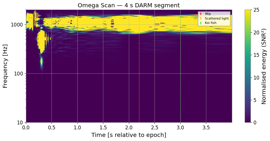
3. Time-Frequency Map (Omega Scan Plot)

QGram.interpolate() resamples the irregular Q tiles onto a regular time-frequency grid suitable for imshow.

# Interpolate to a regular (time, freq) grid
# duration and sampling control the output resolution
qscan_interp = qgram.interpolate(1.0/fs, 1.0)

fig, ax = plt.subplots(figsize=(10, 5))
im = ax.imshow(
    qscan_interp.T,
    origin="lower",
    aspect="auto",
    extent=[t[0], t[-1], 10, 2000],
    vmin=0, vmax=25,
    cmap="viridis",
)
ax.set_yscale("log")
ax.set_xlabel("Time [s relative to epoch]")
ax.set_ylabel("Frequency [Hz]")
ax.set_title("Omega Scan — 4 s DARM segment")

cb = plt.colorbar(im, ax=ax)
cb.set_label("Normalised energy (SNR²)")

# Annotate glitch locations
ax.axvline(t_blip, color="red",   ls="--", lw=1, alpha=0.7, label="Blip")
ax.axvline(2.2,    color="orange", ls="--", lw=1, alpha=0.7, label="Scattered light")
ax.axvline(t_koi,  color="lime",   ls="--", lw=1, alpha=0.7, label="Koi fish")
ax.legend(fontsize=8, loc="upper right")

plt.tight_layout()
plt.show()

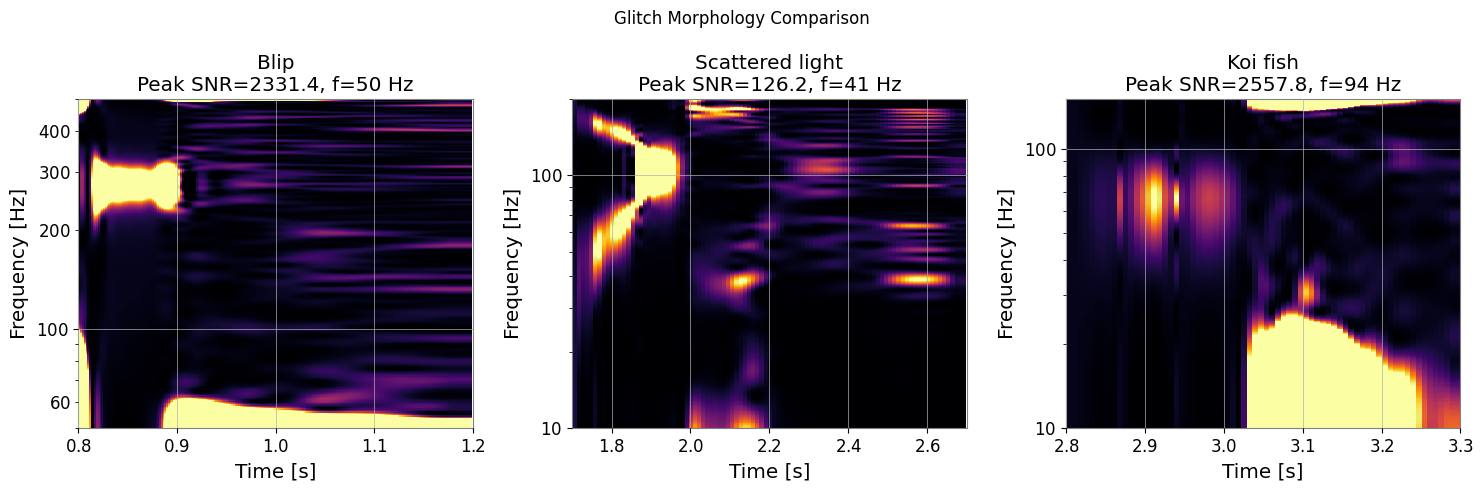
4. Glitch Characterisation with QTiling

QTiling lets us search a specific Q plane and extract glitch parameters (peak time, frequency, duration, bandwidth) for each candidate event.

# Search around each expected glitch location
glitch_windows = [
    ("Blip",            0.8,  1.2,  50,  500, (4,  20)),
    ("Scattered light", 1.7,  2.7,  10,  200, (4,  16)),
    ("Koi fish",        2.8,  3.3,  10,  150, (16, 64)),
]

fig, axes = plt.subplots(1, 3, figsize=(15, 5))

for ax, (name, t_lo, t_hi, f_lo, f_hi, qr) in zip(axes, glitch_windows):
    # Extract sub-segment
    i0, i1 = int(t_lo*fs), int(t_hi*fs)
    ts_seg = TimeSeries(ts_white.value[i0:i1], t0=t0+t_lo,
                        sample_rate=fs, name=name)

    qg, _ = q_scan(ts_seg, qrange=qr, frange=(f_lo, f_hi), mismatch=0.15)
    qi = qg.interpolate(2.0/fs, 2.0)

    ax.imshow(qi.T, origin="lower", aspect="auto", cmap="inferno",
              extent=[t_lo, t_hi, f_lo, f_hi], vmin=0, vmax=20)
    ax.set_yscale("log")
    ax.set_xlabel("Time [s]")
    ax.set_ylabel("Frequency [Hz]")
    ax.set_title(f"{name}\nPeak SNR={qg.peak['energy']:.1f}, "
                 f"f={qg.peak['frequency']:.0f} Hz")

plt.suptitle("Glitch Morphology Comparison", fontsize=12)
plt.tight_layout()
plt.show()

5. Statistical Significance — Rayleigh Test

The rayleigh_test measures how non-Gaussian the time-frequency energy distribution is. A p-value below 0.01 in a quiet background suggests the data segment contains a significant non-Gaussian transient.

# Compare a clean segment vs. a glitchy segment
ts_clean = TimeSeries(noise, t0=t0, sample_rate=fs, name="clean")
ts_clean_w = ts_clean.whiten(fftlength=1.0)
ts_glitch_w = ts_white

qg_clean,  _ = q_scan(ts_clean_w,  qrange=(4,64), frange=(20,500))
qg_glitch, _ = q_scan(ts_glitch_w, qrange=(4,64), frange=(20,500))

# Rayleigh test on normalised energies across tiles
# (simulated as white chi-squared background)
# interpolate QGram to regular grid first, then extract energy values
_qi_clean  = qg_clean.interpolate(1.0/fs, 2.0)
_qi_glitch = qg_glitch.interpolate(1.0/fs, 2.0)
energies_clean  = np.clip(_qi_clean.value.ravel(),  0, None)
energies_glitch = np.clip(_qi_glitch.value.ravel(), 0, None)

r_clean  = rayleigh_test(energies_clean[energies_clean  > 0])
r_glitch = rayleigh_test(energies_glitch[energies_glitch > 0])

print(f"Clean segment  — Rayleigh statistic: {r_clean.statistic:.4f}, "
      f"p-value: {r_clean.pvalue:.4f}")
print(f"Glitchy segment — Rayleigh statistic: {r_glitch.statistic:.4f}, "
      f"p-value: {r_glitch.pvalue:.6f}")
print()
if r_glitch.pvalue < 0.01:
    print("Non-Gaussian transient detected (p < 0.01)")
else:
    print("Segment appears Gaussian at 1% level")

Clean segment  — Rayleigh statistic: 0.4346, p-value: 0.0000
Glitchy segment — Rayleigh statistic: 0.9220, p-value: 0.000000

Non-Gaussian transient detected (p < 0.01)

Summary

Step	API	Output
Whiten data	whiten(ts, fftlength, overlap)	Whitened TimeSeries
Q-scan	q_scan(ts, qrange, frange, mismatch)	QGram, FAR
Plot Omega scan	qgram.interpolate(dt, df)	2D energy array
Glitch parameters	qgram.peak	time, frequency, SNR, Q
Statistical test	rayleigh_test(energies)	statistic, p-value

Glitch morphology guide:

Type	Frequency sweep	Duration	Q range
Blip	None	< 10 ms	4–20
Scattered light	Arch / inverted arch	0.1–1 s	4–16
Koi fish	Low-freq + harmonics	50–200 ms	16–64
Whistle	Monotone sweep	0.1–2 s	20–100

Tip: For production glitch cataloguing, use q_scan with the default qrange=(4,64) and then manually inspect tiles with SNR > 8.