Note
This page was generated from a Jupyter Notebook. Download the notebook (.ipynb)
[1]:
# Skipped in CI: Colab/bootstrap dependency install cell.
Fitting: Basics
Goal: Learn how to fit models to GW data using Ordinary Least Squares (OLS) and Generalized Least Squares (GLS).
GWexpy uses iminuit as its primary optimization engine and provides specialized cost functions for spectral data with correlations.
1. Simple OLS Fit
We start with a simple power-law fit using diagonal errors (OLS).
[2]:
import warnings

warnings.filterwarnings("ignore", category=UserWarning)
warnings.filterwarnings("ignore", category=DeprecationWarning)

import matplotlib.pyplot as plt
import numpy as np

from gwexpy.fitting import fit_series

# Generate synthetic data
freqs = np.linspace(10, 100, 50)
model = lambda f, a, b: a * f + b
y_true = model(freqs, 2.0, 10.0)
y_obs = y_true + np.random.normal(0, 2, size=len(freqs))

from gwexpy.frequencyseries import FrequencySeries

psd = FrequencySeries(y_obs, frequencies=freqs)

res = fit_series(psd, model, p0={"a": 1.0, "b": 1.0})

res.plot()
plt.show()
print(f"Fitted a={res.params['a']:.2f}, b={res.params['b']:.2f}")
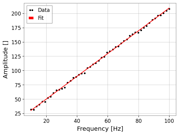
Fitted a=2.00, b=9.58
2. Generalized Least Squares (GLS)
When data points are correlated (e.g., in a PSD estimate with overlapping windows), we use the covariance matrix \(\Sigma\).
[3]:
from iminuit import Minuit

from gwexpy.fitting import GeneralizedLeastSquares

# Create a dummy covariance matrix
cov = np.eye(len(freqs)) * 4.0
cov_inv = np.linalg.inv(cov)

# 1. Define Cost Function
cost = GeneralizedLeastSquares(freqs, y_obs, cov_inv, model, cov=cov)

# 2. Initialize and Run Minuit
m = Minuit(cost, a=1.0, b=1.0)
m.migrad()

print(m.values)
<ValueView a=2.0031926780929914 b=9.578604122772038>
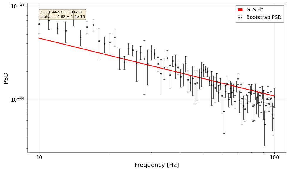
3. High-level Integration
In real analysis, we often estimate the covariance matrix from the data itself using bootstrap methods. GWexpy provides an integrated pipeline for this.
[4]:
from gwexpy.fitting.highlevel import fit_bootstrap_spectrum
from gwexpy.noise.wave import colored

# Generate 10 seconds of pink noise
data = colored(duration=10, sample_rate=256, exponent=0.5, amplitude=1e-21)

def power_law(f, A, alpha):
    return A * f**alpha

result = fit_bootstrap_spectrum(
    data,
    model_fn=power_law,
    freq_range=(10, 100),
    fftlength=1.0,
    overlap=0.5,
    initial_params={"A": 1e-21, "alpha": -0.5},
    plot=True
)
4. Exercises
Parameter Bounds: Modify the OLS fit to restrict
a > 0using thelimitsargument infit_series.MCMC: Enable MCMC in Section 3 by setting
run_mcmc=True(requiresemcee).
5. Quick Check (NBMAKE)
[5]:
assert "a" in res.params
assert result.reduced_chi2 > 0
print("Validation successful!")
Validation successful!