FrequencySeries: 基本#
このノートブックでは、gwexpy で拡張された FrequencySeries クラスの新しいメソッドと機能について紹介します。 主に複素スペクトルの扱い、微積分、フィルタリング(スムージング)、および他ライブラリとの連携機能に焦点を当てます。
import warnings


import matplotlib.pyplot as plt
import numpy as np

from gwexpy.frequencyseries import FrequencySeries
from gwexpy.plot import Plot
from gwexpy.timeseries import TimeSeries

plt.rcParams["figure.figsize"] = (10, 6)
1. データの準備#
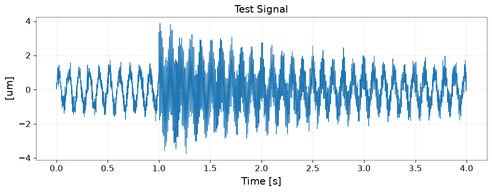
まずは TimeSeries から FFT を用いて FrequencySeries を作成します。 ここでは、特定の周波数成分を持つテスト信号を生成します。
fs = 1024
t = np.arange(0, 4, 1 / fs)
exp = np.exp(-t / 1.5)
exp[: int(exp.size / 4)] = 0
data = (
    np.sin(2 * np.pi * 10.1 * t)
    + 5 * exp * np.sin(2 * np.pi * 100.1 * t)
    + np.random.normal(scale=0.3, size=len(t))
)
ts = TimeSeries(data, dt=1 / fs, unit="um", name="Test Signal")
print(ts)

fig, ax = plt.subplots(figsize=(10, 4))
ax.plot(ts.times.value, ts.value, lw=0.8)
ax.set_xlabel("Time [s]")
ax.set_ylabel(f"[{ts.unit}]")
ax.set_title(ts.name)
ax.grid(True, alpha=0.3)
plt.tight_layout()
plt.show()

# Perform FFT to obtain FrequencySeries (using transient mode with padding)
spec = ts.fft(mode="transient", pad_left=1.0, pad_right=1.0, nfft_mode="next_fast_len")
print(f"Type: {type(spec)}")
print(f"Length: {len(spec)}")
print(f"df: {spec.df}")
TimeSeries([0.1455092 , 0.03913578, 0.38809661, ..., 0.2470566 ,
            1.02017138, 1.02172736],
           unit: um,
           t0: 0.0 s,
           dt: 0.0009765625 s,
           name: Test Signal,
           channel: None)
Type: <class 'gwexpy.frequencyseries.frequencyseries.FrequencySeries'>
Length: 3073
df: 0.16666666666666666 Hz
2. 複素スペクトルの可視化と変換#
位相と振幅#
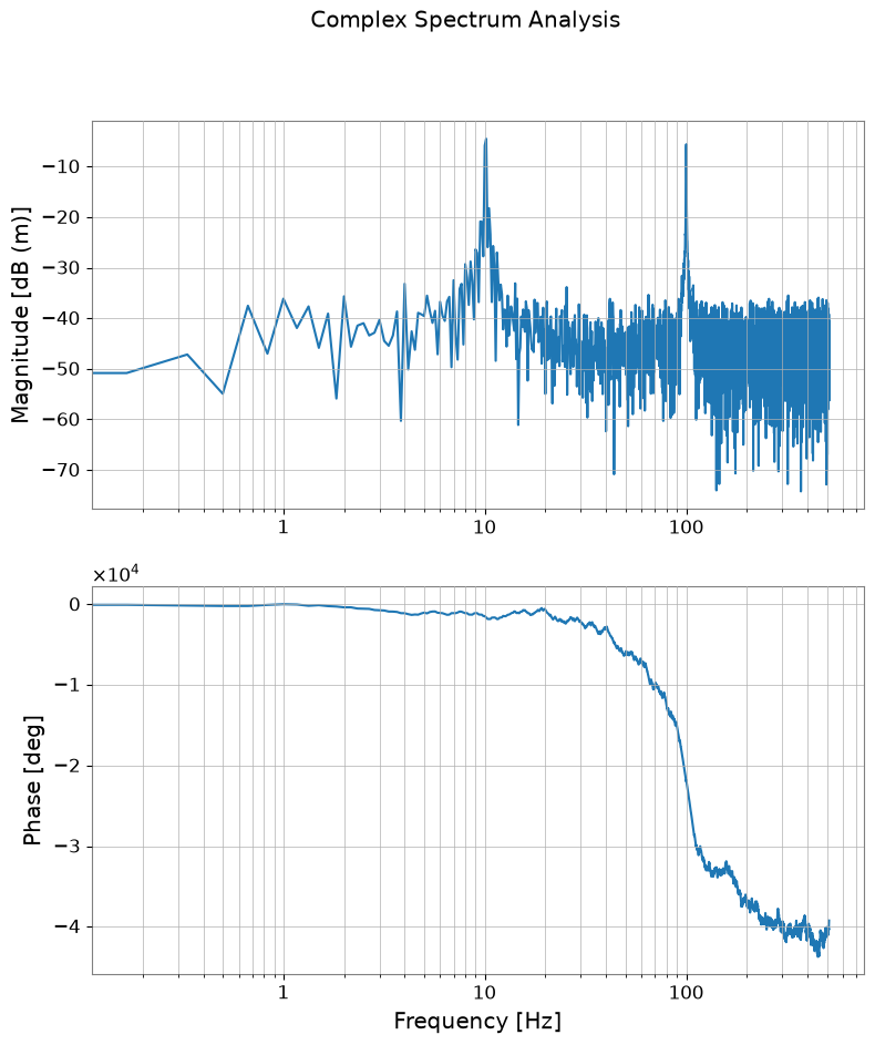
phase(), degree(), to_db() メソッドを使用すると、複素スペクトルを直感的な単位に変換できます。
# Convert amplitude to dB (ref=1.0, 20*log10)
spec_db = spec.to_db()

# Get phase (in degrees, unwrap=True for continuity)
spec_phase = spec.degree(unwrap=True)

plot = Plot(spec_db, spec_phase, separate=True, sharex=True, xscale="log")
ax = plot.axes
ax[0].set_ylabel("Magnitude [dB (m)]")
ax[0].grid(True, which="both")

ax[1].set_ylabel("Phase [deg]")
ax[1].set_xlabel("Frequency [Hz]")
ax[1].grid(True, which="both")
plot.figure.suptitle("Complex Spectrum Analysis")
plot.show()
3. 周波数ドメインでの微積分#
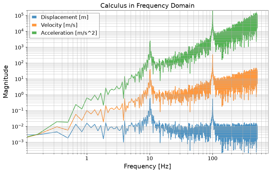
differentiate() および integrate() メソッドにより、周波数ドメインで微分・積分を行うことができます。 引数 order で階数を指定できます(デフォルトは1)。 これは「変位・速度・加速度」の変換(\((2 \pi i f)^n\) の乗算・除算)を簡単に行うための機能です。
# Differentiate from displacement (m) to velocity (m/s) (order=1)
vel_spec = spec.differentiate()

# Differentiate from displacement (m) to acceleration (m/s^2) (order=2)
accel_spec = spec.differentiate(order=2)

# Integration is also possible: acceleration -> velocity
vel_from_accel = accel_spec.integrate()

plot = Plot(
    spec.abs(), vel_spec.abs(), accel_spec.abs(), xscale="log", yscale="log", alpha=0.8
)
ax = plot.gca()
ax.get_lines()[0].set_label("Displacement [m]")
ax.get_lines()[1].set_label("Velocity [m/s]")
ax.get_lines()[2].set_label("Acceleration [m/s^2]")
ax.legend()
ax.grid(True, which="both")
ax.set_title("Calculus in Frequency Domain")
ax.set_ylabel("Magnitude")
plot.show()
4. スペクトルのスムージングとピーク検出#
スムージング#
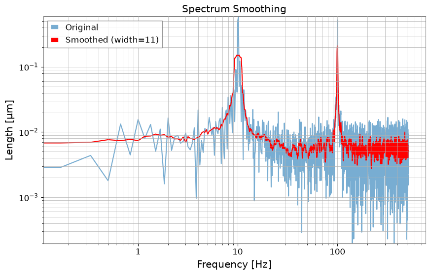
smooth() メソッドを使用すると、移動平均などによるスペクトルの平滑化が可能です。
# Smooth in amplitude domain with 11 samples
spec_smooth = spec.smooth(width=11)

plot = Plot(spec.abs(), spec_smooth.abs(), xscale="log", yscale="log")
ax = plot.gca()
ax.get_lines()[0].set_label("Original")
ax.get_lines()[0].set_alpha(0.6)
ax.get_lines()[1].set_label("Smoothed (width=11)")
ax.get_lines()[1].set_color("red")
ax.legend()
ax.grid(True, which="both")
ax.set_title("Spectrum Smoothing")
plot.show()
ピーク検出#
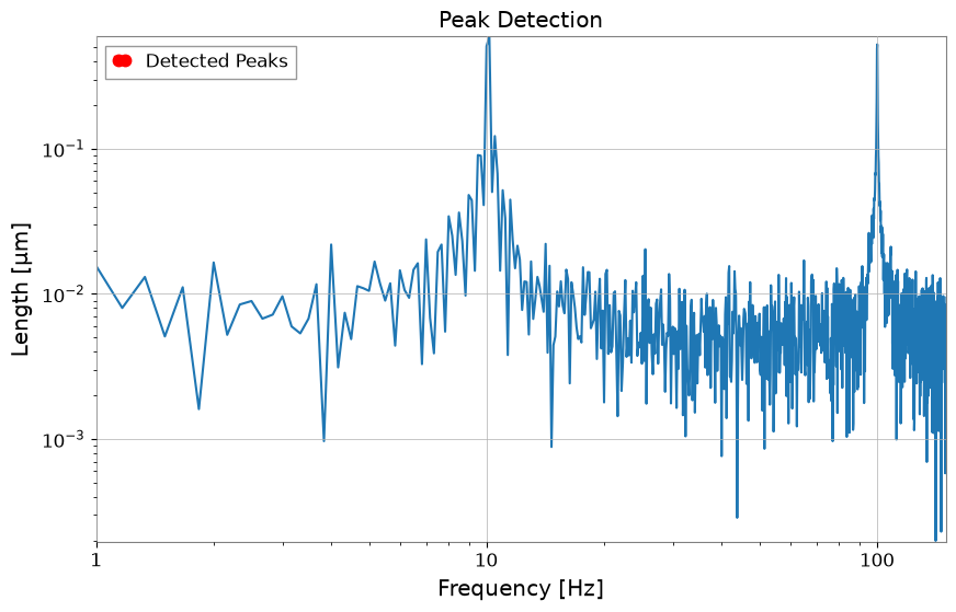
find_peaks() メソッドは scipy.signal.find_peaks をラップしており、特定の閾値を超えるピークを簡単に抽出できます。
# Find peaks with amplitude >= 0.2
peaks, props = spec.find_peaks(threshold=0.2)

plot = Plot(spec.abs())
ax = plot.gca()
ax.plot(
    peaks.abs(), color="red", marker=".", ms=15, lw=0, zorder=3, label="Detected Peaks"
)
ax.set_xlim(1, 150)
ax.set_xscale("log")
ax.set_yscale("log")
ax.set_title("Peak Detection")
ax.legend()
plot.show()
5. 高度な解析機能#
群遅延 (Group Delay)#
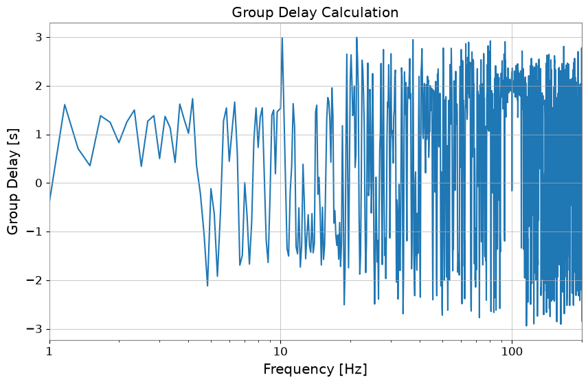
group_delay() メソッドは、位相の周波数微分から群遅延(信号のエンベロープの遅延)を計算します。
gd = spec.group_delay()

plot = Plot(gd)
ax = plot.gca()
ax.set_ylabel("Group Delay [s]")
ax.set_xlabel("Frequency [Hz]")
ax.set_xlim(1, 200)
ax.set_title("Group Delay Calculation")
plot.show()
逆FFT (ifft)#
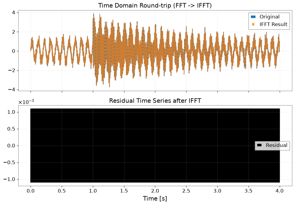
ifft() メソッドは、TimeSeries を返します。mode="transient" で FFT した結果であっても、情報を引き継いで元の長さに戻す (trim=True) などの制御が可能です。
# Convert back to TimeSeries with inverse FFT
# mode="auto" reads the transient information from the input FrequencySeries and processes it appropriately
inv_ts = spec.ifft(mode="auto")
red_ts = inv_ts - ts

fig, axes = plt.subplots(2, 1, figsize=(10, 7), sharex=True)
axes[0].plot(ts.times.value, ts.value, label="Original")
axes[0].plot(inv_ts.times.value, inv_ts.value, "--", alpha=0.8, label="IFFT Result")
axes[0].set_title("Time Domain Round-trip (FFT -> IFFT)")
axes[0].legend()
axes[0].grid(True, alpha=0.3)

axes[1].plot(red_ts.times.value, red_ts.value, color="black", label="Residual")
axes[1].set_title("Residual Time Series after IFFT")
axes[1].set_xlabel("Time [s]")
axes[1].legend()
axes[1].grid(True, alpha=0.3)

plt.tight_layout()
plt.show()
6. 他ライブラリとの連携#
Pandas, xarray, control ライブラリとの相互変換が追加されています。
# Convert to Pandas Series
pd_series = spec.to_pandas()
print("Pandas index sample:", pd_series.index[:5])
display(pd_series)

# Convert to xarray DataArray
try:
    da = spec.to_xarray()
    print("xarray coord name:", list(da.coords))
    display(da)
except ImportError:
    print("xarray not installed, skipping DataArray conversion.")

# Convert to control.FRD (can be used for control system analysis)
try:
    from control import FRD

    _ = FRD
    frd_obj = spec.to_control_frd()
    print("Successfully converted to control.FRD")
    display(frd_obj)
except ImportError:
    print("python-control library not installed")
Pandas index sample: Index([0.0, 0.16666666666666666, 0.3333333333333333, 0.5, 0.6666666666666666], dtype='float64', name='frequency')
frequency
0.000000      0.005283+0.000000j
0.166667      0.001442-0.002486j
0.333333     -0.003555-0.002563j
0.500000     -0.001649+0.000704j
0.666667     -0.012250+0.005167j
                     ...
511.333333    0.004898-0.003660j
511.500000   -0.003551+0.003280j
511.666667    0.000965-0.001186j
511.833333   -0.001880-0.001731j
512.000000    0.002182+0.000000j
Name: Test Signal, Length: 3073, dtype: complex128
xarray coord name: ['frequency']
<xarray.DataArray 'Test Signal' (frequency: 3073)> Size: 49kB
array([ 0.00528306+0.j        ,  0.00144241-0.00248599j,
       -0.00355532-0.00256334j, ...,  0.00096527-0.0011863j ,
       -0.00188018-0.00173084j,  0.00218154+0.j        ],
      shape=(3073,))
Coordinates:
  * frequency  (frequency) float64 25kB 0.0 0.1667 0.3333 ... 511.7 511.8 512.0
Attributes:
    unit:     um
epoch: 0.0Successfully converted to control.FRD
FrequencyResponseData(
array([[[ 0.00528306+0.j        ,  0.00144241-0.00248599j,
         -0.00355532-0.00256334j, ...,
          0.00096527-0.0011863j , -0.00188018-0.00173084j,
          0.00218154+0.j        ]]], shape=(1, 1, 3073)),
array([0.00000000e+00, 1.66666667e-01, 3.33333333e-01, ...,
       5.11666667e+02, 5.11833333e+02, 5.12000000e+02],
      shape=(3073,)),
outputs=1, inputs=1)
7. Python Control Library との連携#
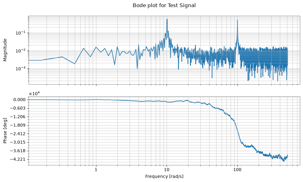
制御工学の分野で標準的な control ライブラリの Frequency Response Data (FRD) オブジェクトと相互変換が可能です。 これにより、GWexpyで計測した伝達関数を、制御系の設計や解析に直接利用できます。
try:
    import control

    # Convert FrequencySeries -> control.FRD
    # Specifying frequency_unit="Hz" appropriately converts to rad/s internally
    frd_sys = spec.to_control_frd(frequency_unit="Hz")

    print("\n--- Converted to Control FRD ---")
    print(str(frd_sys)[:1000] + "\n... (truncated) ...")

    # Plot Bode diagram (control library functionality)
    control.bode(frd_sys)  # (executable if plotting environment is available)

    # Restore control.FRD -> FrequencySeries
    fs_restored = FrequencySeries.from_control_frd(frd_sys, frequency_unit="Hz")

    print("\n--- Restored FrequencySeries ---")
    print(fs_restored)

except ImportError:
    print("Python Control Systems Library is not installed.")
--- Converted to Control FRD ---
<FrequencyResponseData>: sys[1]
Inputs (1): ['u[0]']
Outputs (1): ['y[0]']

Freq [rad/s]  Response
------------  ---------------------
       0.000    0.005283        +0j
       0.167    0.001442 -0.002486j
       0.333   -0.003555 -0.002563j
       0.500   -0.001649+0.0007043j
       0.667    -0.01225 +0.005167j
       0.833    0.001465 -0.004221j
       1.000     0.01515 +0.003784j
       1.167    0.007464 -0.002911j
       1.333     -0.0131-0.0001182j
       1.500   -0.001399 -0.004901j
       1.667   -0.008235 +0.007479j
       1.833   5.523e-05 +0.001608j
       2.000     0.01611 -0.003456j
       2.167    0.005123 -0.001046j
       2.333   -0.008089 -0.002469j
       2.500   -0.008751 +0.001811j
       2.667   -0.006154 +0.002787j
       2.833     0.00694 +0.001932j
       3.000     0.00948  -0.00177j
       3.167    0.004235 -0.004213j
       3.333    -0.00533-0.0004594j
       3.500    -0.00676+0.0001127j
       3.667   -0.008115 +0.008377j
       3.833   0.0009307-0.0002639j

... (truncated) ...
--- Restored FrequencySeries ---
FrequencySeries([ 0.00528306+0.j        ,
                  0.00144241-0.00248599j,
                 -0.00355532-0.00256334j, ...,
                  0.00096527-0.0011863j ,
                 -0.00188018-0.00173084j,
                  0.00218154+0.j        ],
                unit: dimensionless,
                f0: 0.0 Hz,
                df: 0.02652582384864922 Hz,
                epoch: None,
                name: None,
                channel: None)
8. 求積和 (Quadrature Sum)#
直交位相の和を計算する機能です。
# Generate noisy data
np.random.seed(42)
f = spec.frequencies.value
noise = np.abs(np.random.randn(f.size))
peak = 10.0 * np.exp(-((f - 200) ** 2) / 50.0)
data = noise + peak

raw = FrequencySeries(data, frequencies=f, unit="V", name="Raw Data")

# Smooth
smoothed = raw.smooth(width=10, method="amplitude")
smoothed.name = "Smoothed"

# Convert to dB
raw_db = raw.to_db()
smoothed_db = smoothed.to_db()
raw_db.name = "Raw (dB)"
smoothed_db.name = "Smoothed (dB)"

plot = raw_db.plot(label="Raw", title="Smoothing & dB")
ax = plot.gca()
ax.plot(smoothed_db, label="Smoothed", linewidth=2)
ax.legend()
plot.show()
plt.close()

# Quadrature Sum (Noise Budget example)
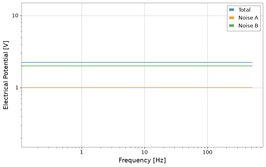
noise_a = FrequencySeries(np.ones_like(f), frequencies=f, unit="V", name="Noise A")
noise_b = FrequencySeries(np.ones_like(f) * 2, frequencies=f, unit="V", name="Noise B")

total = noise_a.quadrature_sum(noise_b)
print(f"Noise A: {noise_a.value[0]}, Noise B: {noise_b.value[0]}")
print(f"Total (Sqrt Sum): {total.value[0]}")
Plot(total, noise_a, noise_b, alpha=0.8)
plt.legend(["Total", "Noise A", "Noise B"])
plt.xscale("log")
plt.yscale("log")
plt.show()
Noise A: 1.0, Noise B: 2.0
Total (Sqrt Sum): 2.23606797749979