
フィッティング: 基本#
目的: 通常最小二乗法(OLS)および一般化最小二乗法(GLS)を使用して GW データにモデルをフィットする方法を学びます。
GWexpy は主要な最適化エンジンとして iminuit を使用し、相関を持つスペクトルデータ用の特化したコスト関数を提供します。
このノートブックを実行する前に、fitting extra でインストールしてください: pip install "gwexpy[fitting]"。
1. 単純な OLS フィット#
対角誤差(OLS)を使った単純なべき乗則フィットから始めます。
import warnings


import matplotlib.pyplot as plt
import numpy as np
np.random.seed(42)

from gwexpy.fitting import fit_series

# Generate synthetic data following a power law: y = A * f**alpha
freqs = np.linspace(10, 100, 50)
model = lambda f, A, alpha: A * f**alpha
y_true = model(freqs, 1000.0, -1.5)
y_obs = y_true + np.random.normal(0, 0.3, size=len(freqs))

from gwexpy.frequencyseries import FrequencySeries

psd = FrequencySeries(y_obs, frequencies=freqs)

res = fit_series(psd, model, p0={"A": 100.0, "alpha": -1.0})

res.plot()
plt.xscale("log")
plt.yscale("log")
plt.show()
print(f"Fitted A={res.params['A']:.2f}, alpha={res.params['alpha']:.2f}")
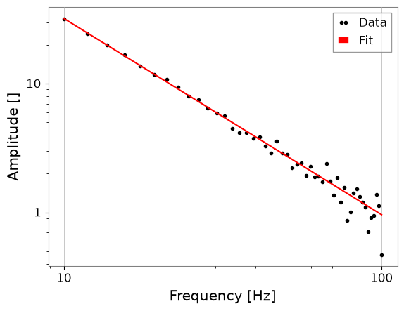
Fitted A=1063.49, alpha=-1.52
2. 一般化最小二乗法(GLS)#
データ点が相関している場合(例:重なり窓を使った PSD 推定)、共分散行列 \(\Sigma\) を使用します。
from iminuit import Minuit

from gwexpy.fitting import GeneralizedLeastSquares

# Build a correlated (non-diagonal) covariance matrix: Sigma_ij = sigma^2 * rho^|i-j|
sigma = 2.0
rho = 0.6
idx = np.arange(len(freqs))
cov = sigma**2 * rho ** np.abs(idx[:, None] - idx[None, :])
cov_inv = np.linalg.inv(cov)

# Resample data with correlated noise drawn directly from this covariance
y_obs_corr = np.random.multivariate_normal(y_true, cov)

# 1. Define Cost Function
cost = GeneralizedLeastSquares(freqs, y_obs_corr, cov_inv, model, cov=cov)

# 2. Initialize and Run Minuit
m = Minuit(cost, A=100.0, alpha=-1.0)
m.migrad()

print("GLS fit (accounts for the correlated noise):")
print(m.values)
print(m.errors)

# Compare against an OLS fit on the *same* data, using the *same* per-point
# variance (the diagonal of `cov`) but ignoring the off-diagonal correlation.
# This isolates the effect of the correlation alone.
sigma_diag = np.sqrt(np.diag(cov))
psd_corr = FrequencySeries(y_obs_corr, frequencies=freqs)
res_ols_on_corr = fit_series(
    psd_corr, model, sigma=sigma_diag, p0={"A": 100.0, "alpha": -1.0}
)

print("\nOLS fit on the same data using only the diagonal of `cov` (ignores correlation):")
print(
    f"  A={res_ols_on_corr.params['A']:.3f} +/- {res_ols_on_corr.errors['A']:.3f}, "
    f"alpha={res_ols_on_corr.params['alpha']:.3f} +/- {res_ols_on_corr.errors['alpha']:.3f}"
)
print(
    f"  GLS: A={m.values['A']:.3f} +/- {m.errors['A']:.3f}, "
    f"alpha={m.values['alpha']:.3f} +/- {m.errors['alpha']:.3f}"
)
GLS fit (accounts for the correlated noise):
<ValueView A=908.960879383731 alpha=-1.4988207218966207>
<ErrorView A=332.11791032869723 alpha=0.14281485260130117>

OLS fit on the same data using only the diagonal of `cov` (ignores correlation):
  A=860.762 +/- 205.568, alpha=-1.481 +/- 0.087
  GLS: A=908.961 +/- 332.118, alpha=-1.499 +/- 0.143
上記の 2 つのフィットは、いずれも同じ y_obs_corr データ、同じモデル、同じ各点の観測誤差(cov の対角成分の平方根である sigma_diag)を使用しています。OLS フィットは共分散の対角成分のみを使い、GLS フィットは非対角の相関項を含む共分散全体を使うため、両者の違いは相関を考慮するかどうかだけであり、各点の誤差の大きさの前提は同じです。m.errors と res_ols_on_corr.errors は、いずれも最小二乗コスト関数(errordef = Minuit.LEAST_SQUARES = 1.0)のもとで iminuit が計算する Hesse 近似による不確かさなので、直接比較できます。
この相関構造とこの1回のデータの実現では、GLS フィットは相関を無視した OLS フィットよりも A と alpha の両方で不確かさを大きく見積もります。これは、相関のあるノイズを独立とみなすと OLS が不確かさを過小評価するという説明と整合します。ただし、これは1回の実現に基づく結果であり、統計的な保証ではありません。より厳密な検証には、多数回の乱数試行にわたるパラメータ回収の精度や信頼区間の被覆率を調べる必要がありますが、それは本入門教材の範囲を超えます。
3. 高レベル統合パイプライン#
実際の解析では、ブートストラップ法を使ってデータ自体から共分散行列を推定することが多いです。GWexpy はこのための統合パイプラインを提供しています。
from gwexpy.fitting.highlevel import fit_bootstrap_spectrum
from gwexpy.noise.wave import colored

# Generate 10 seconds of pink noise
data = colored(duration=10, sample_rate=256, exponent=0.5, amplitude=1e-21)

def power_law(f, A, alpha):
    return A * f**alpha

result = fit_bootstrap_spectrum(
    data,
    model_fn=power_law,
    freq_range=(10, 100),
    fftlength=1.0,
    overlap=0.5,
    initial_params={"A": 1e-21, "alpha": -0.5},
    plot=True
)
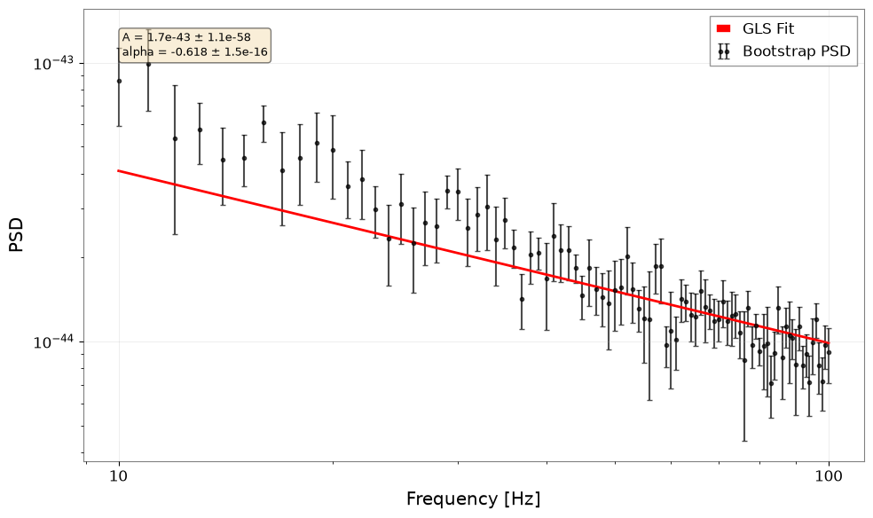
4. 演習#
パラメータ制約:
fit_seriesのlimits引数を使ってA > 0となるよう OLS フィットを修正してください。MCMC: セクション 3 で
run_mcmc=Trueを設定して MCMC を有効にしてください(emceeが必要)。
5. 検証セル(NBMAKE)#
assert "A" in res.params
assert result.reduced_chi2 > 0
print("Validation successful!")
Validation successful!