Note

This page was generated from a Jupyter Notebook. Download the notebook (.ipynb)

# Skipped in CI: Colab/bootstrap dependency install cell.

Control Analysis: Plant Modeling from Measured Response

This notebook promotes the legacy system-identification example into the public tutorial set. The modeling step matters because a controller should be designed against the part of the response that is both physically meaningful and measured with high coherence.

We regenerate a resonant plant, estimate its transfer function, select a trustworthy frequency range, and fit a compact second-order model.

import matplotlib.pyplot as plt
import numpy as np
import scipy.signal as signal
from control.matlab import bode, tf
from scipy.optimize import curve_fit

from gwexpy import TimeSeries

fs = 1024
duration = 60
t = np.arange(0, duration, 1 / fs)

f0_true = 10.0
Q_true = 10.0
w0_true = 2 * np.pi * f0_true
num_true = [w0_true**2]
den_true = [1, w0_true / Q_true, w0_true**2]

# Broadband excitation plus measured output recreates the experimental data that a control engineer would actually fit.
np.random.seed(42)
u_vals = np.random.randn(len(t))
sys_dt = signal.cont2discrete((num_true, den_true), 1 / fs)
y_vals = signal.dlti(sys_dt[0], sys_dt[1], dt=1 / fs).output(u_vals, t=t)[1].flatten()

u = TimeSeries(u_vals, times=t, unit="V", name="Input")
y = TimeSeries(y_vals, times=t, unit="m", name="Output")

fftlength = 4
tf_meas = y.transfer_function(u, fftlength=fftlength)
coh = y.coherence(u, fftlength=fftlength)

/home/runner/micromamba/envs/gwexpy/lib/python3.11/site-packages/scipy/signal/_ltisys.py:603: BadCoefficients: Badly conditioned filter coefficients (numerator): the results may be meaningless
  self.num, self.den = normalize(*system)

1. Keep only the physically trustworthy band

A good model fit uses frequencies where the plant dominates and the measurement is coherent. Low-coherence points usually indicate noise domination or unmodeled dynamics.

freqs = tf_meas.frequencies.value
mask = (freqs >= 1) & (freqs <= 200) & (coh.value >= 0.9)

f_fit = freqs[mask]
data_fit = tf_meas.value[mask]
print(f"Selected {len(f_fit)} frequency points for fitting.")

Selected 797 frequency points for fitting.

2. Fit a resonator model

The fitted parameters have direct physical meaning: gain sets actuation scale, f0 gives the resonance frequency, and Q gives the damping width.

def model_mag(f, K, f0, Q):
    w = 2 * np.pi * f
    w0 = 2 * np.pi * f0
    return np.abs(K * (w0**2) / ((w0**2) - (w**2) + 1j * w * w0 / Q))

popt, _ = curve_fit(model_mag, f_fit, np.abs(data_fit), p0=[1.0, 10.0, 8.0])
K_fit, f0_fit, Q_fit = popt
print(f"K={K_fit:.3f}, f0={f0_fit:.3f} Hz, Q={Q_fit:.3f}")

K=72.019, f0=189.380 Hz, Q=5.665

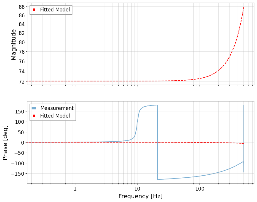
3. Compare the fitted model with the measurement

A credible plant model should match both the peak location and the width of the measured resonance, not just one point on the curve.

w0_fit = 2 * np.pi * f0_fit
sys_fit = tf([K_fit * w0_fit**2], [1, w0_fit / Q_fit, w0_fit**2])
mag_fit, phase_fit, _ = bode(sys_fit, freqs, plot=False)

fig, (ax1, ax2) = plt.subplots(2, 1, sharex=True, figsize=(10, 8))
tf_meas.abs().plot(ax=ax1, label="Measurement", alpha=0.6)
ax1.loglog(freqs, mag_fit, "r--", label="Fitted Model")
ax1.set_ylabel("Magnitude")
ax1.legend()
ax1.grid(True, which="both", alpha=0.5)

phase_meas_deg = np.rad2deg(np.angle(tf_meas.value))
ax2.semilogx(freqs, phase_meas_deg, label="Measurement", alpha=0.6)
ax2.semilogx(freqs, np.rad2deg(phase_fit), "r--", label="Fitted Model")
ax2.set_ylabel("Phase [deg]")
ax2.set_xlabel("Frequency [Hz]")
ax2.legend()
ax2.grid(True, which="both", alpha=0.5)
plt.show()