Note

This page was generated from a Jupyter Notebook. Download the notebook (.ipynb)

Time Series Forecasting with ARIMA Models

This notebook demonstrates how to model and forecast time series data using ARIMA-related functions (AR, MA, ARMA, ARIMA/SARIMAX) that have been added to the gwexpy TimeSeries class.

Setup

Import the necessary libraries.

import warnings

import matplotlib.pyplot as plt
import numpy as np

warnings.filterwarnings(
    "ignore", message=r".*force_all_finite.*", category=FutureWarning
)
warnings.filterwarnings("ignore", category=FutureWarning, module=r"sklearn\..*")
warnings.filterwarnings("ignore", category=FutureWarning, module=r"pmdarima\..*")

from gwexpy.timeseries import TimeSeries

Creating Sample Data

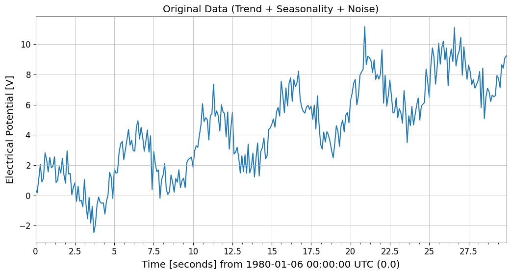
To verify the effectiveness of ARIMA models, we create synthetic data that includes a trend, seasonality (periodicity), and noise.

# Trend + Seasonality + Noise
t0 = 0
dt = 0.1
duration = 30
t = np.arange(0, duration, dt)
n_samples = len(t)

# 1. Linear Trend
trend = 0.3 * t

# 2. Periodic component (Sine)
seasonality = 2.0 * np.sin(2 * np.pi * 0.2 * t)

# 3. Noise
np.random.seed(42)
noise = np.random.normal(0, 0.8, n_samples)

data = trend + seasonality + noise

# Create TimeSeries object
ts = TimeSeries(data, t0=t0, dt=dt, unit="V", name="Sample Data")

ts.plot()
plt.title("Original Data (Trend + Seasonality + Noise)")
plt.show()

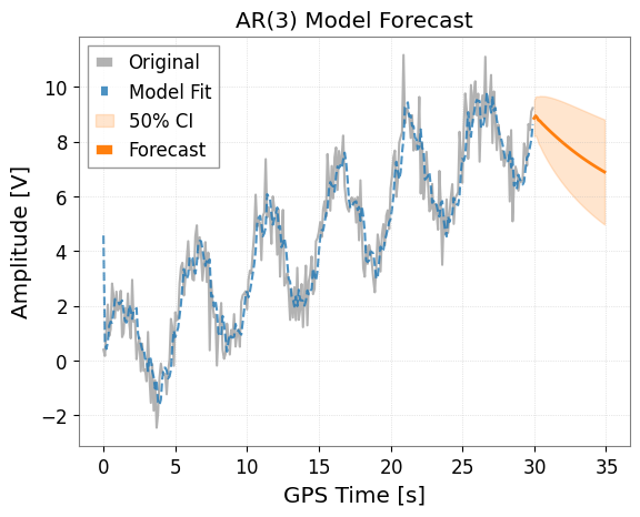
1. AR (AutoRegressive) Model

The AR model assumes that the current value depends on past values. Use the ts.ar(p) method, where p is the order.

# Fit with order p=3
model_ar = ts.ar(p=3)

# Display model summary
# print(model_ar.summary())

# Plot results
# forecast_steps specifies how many steps to forecast into the future
model_ar.plot(forecast_steps=50, alpha=0.5)
plt.title("AR(3) Model Forecast")
plt.show()

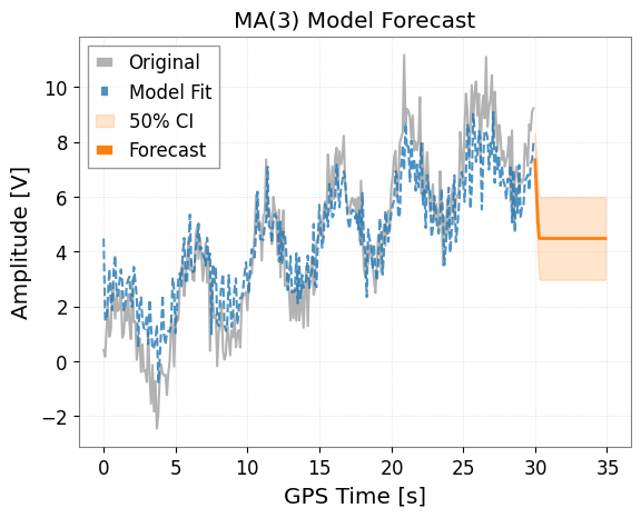
2. MA (Moving Average) Model

The MA model assumes that the current value depends on past prediction errors (white noise). Use the ts.ma(q) method.

# Fit with order q=3
model_ma = ts.ma(q=3)

# Plot results
model_ma.plot(forecast_steps=50, alpha=0.5)
plt.title("MA(3) Model Forecast")
plt.show()

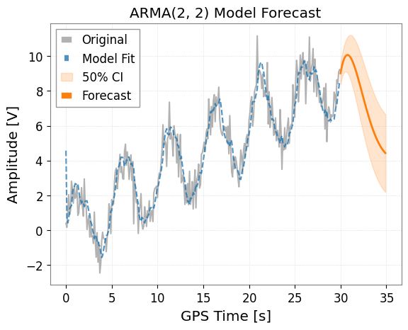
3. ARMA (AutoRegressive Moving Average) Model

The ARMA model combines AR and MA. Use the ts.arma(p, q) method.

# Fit with p=2, q=2
model_arma = ts.arma(p=2, q=2)

model_arma.plot(forecast_steps=50, alpha=0.5)
plt.title("ARMA(2, 2) Model Forecast")
plt.show()

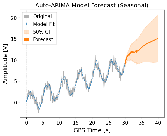
4. ARIMA / Auto-ARIMA

The ARIMA model removes non-stationarity (such as trends) by differencing, then applies the ARMA model.

Use the ts.arima() method. With the auto=True option, the pmdarima library is used to automatically search for optimal parameters (p, d, q). This is the most recommended approach.

try:
    print("Searching for optimal ARIMA parameters... (this may take a few seconds)")

    # Seasonality can also be considered
    # m is the number of steps in a seasonal period
    model_auto = ts.arima(auto=True, auto_kwargs={"seasonal": True, "m": 50})

    # Show info of the optimal model found
    print(model_auto.summary())

    # Plot results (Forecasting for a longer period)
    ax = model_auto.plot(forecast_steps=100, alpha=0.5)
    plt.title("Auto-ARIMA Model Forecast (Seasonal)")
    plt.show()
except ImportError as e:
    print(f"Auto-ARIMA skipping: {e}")

Searching for optimal ARIMA parameters... (this may take a few seconds)
                                      SARIMAX Results
===========================================================================================
Dep. Variable:                                   y   No. Observations:                  300
Model:             SARIMAX(1, 1, 2)x(1, 0, [], 50)   Log Likelihood                -404.141
Date:                             Thu, 26 Feb 2026   AIC                            820.282
Time:                                     20:48:31   BIC                            842.485
Sample:                                          0   HQIC                           829.169
                                             - 300
Covariance Type:                               opg
==============================================================================
                 coef    std err          z      P>|z|      [0.025      0.975]
------------------------------------------------------------------------------
intercept      0.0044      0.006      0.695      0.487      -0.008       0.017
ar.L1          0.8693      0.053     16.310      0.000       0.765       0.974
ma.L1         -1.6277      0.052    -31.464      0.000      -1.729      -1.526
ma.L2          0.7409      0.043     17.235      0.000       0.657       0.825
ar.S.L50       0.1604      0.071      2.263      0.024       0.021       0.299
sigma2         0.8667      0.070     12.431      0.000       0.730       1.003
===================================================================================
Ljung-Box (L1) (Q):                   0.13   Jarque-Bera (JB):                 0.69
Prob(Q):                              0.71   Prob(JB):                         0.71
Heteroskedasticity (H):               1.37   Skew:                            -0.10
Prob(H) (two-sided):                  0.12   Kurtosis:                         3.14
===================================================================================

Warnings:
[1] Covariance matrix calculated using the outer product of gradients (complex-step).

5. Obtaining Forecast Data

Beyond plotting, you can directly obtain forecast values as a TimeSeries object using the .forecast() method. This also includes confidence intervals.

if "model_auto" not in dir():
    print("Auto-ARIMA model not available (pmdarima may be missing); skipping forecast.")
else:
    steps = 50

    # Get forecast values and confidence intervals
    forecast_ts, intervals = model_auto.forecast(
        steps=steps, alpha=0.5
    )  # 50% confidence interval

    print("Forecast Data:")
    print(forecast_ts)

    print("\nConfidence Interval (Upper):")
    print(intervals["upper"])

    # Forecasting data can be saved or used for other analysis
    # forecast_ts.write("forecast.h5")

Forecast Data:
TimeSeries([ 9.02063095,  9.60946546, 10.04247608, 10.15366724,
            10.05259678, 10.38953409, 10.79815095, 10.71027742,
            11.00660771, 11.18205177, 11.08230487, 11.29883005,
            10.98339795, 11.34916921, 11.51885662, 11.45196033,
            11.87327376, 11.52379092, 11.68683663, 11.78939387,
            11.98098394, 11.6301629 , 11.97773482, 11.84042886,
            11.72116368, 11.91254849, 11.88390198, 11.78617506,
            11.8774454 , 11.82552207, 11.89784228, 11.97900471,
            12.11133126, 11.76628355, 12.22002271, 11.72134704,
            11.98239983, 12.11216074, 12.11237757, 12.04095272,
            12.1435007 , 12.16098299, 12.2071204 , 12.45443501,
            12.45772066, 12.39288272, 12.67001284, 12.66918601,
            12.8110433 , 12.8657357 ],
           unit: V,
           t0: 30.0 s,
           dt: 0.1 s,
           name: Sample Data_auto_forecast,
           channel: None)

Confidence Interval (Upper):
TimeSeries([ 9.64857296, 10.25546653, 10.7195876 , 10.87456042,
            10.82818582, 11.22844355, 11.7067511 , 11.69299174,
            12.06629413, 12.32035964, 12.29997326, 12.59592369,
            12.35948866, 12.80347361, 13.05033984, 13.05941406,
            13.55537472, 13.27914473, 13.51401064, 13.68694154,
            13.94746299, 13.66414849, 14.07782921, 14.0052681 ,
            13.9494223 , 14.20294246, 14.23519045, 14.19716117,
            14.34697639, 14.35248881, 14.48117848, 14.61768579,
            14.80437308, 14.51274095, 15.01898802, 14.57194853,
            14.88380013, 15.06355532, 15.11299318, 15.09004592,
            15.24035641, 15.30491312, 15.39746251, 15.69055103,
            15.73899569, 15.71872387, 16.03984813, 16.08246334,
            16.26722947, 16.36431549],
           unit: V,
           t0: 30.0 s,
           dt: 0.1 s,
           name: upper_ci,
           channel: None)

6. Application in Gravitational Wave Data Analysis: Noise Removal (Whitening) with ARIMA

In gravitational wave data analysis, a process called whitening is performed to extract burst signals or ringdown waveforms from stationary “colored noise”. By training an ARIMA model as a predictive model for background noise and subtracting the predicted values from the measured values (taking residuals), it is possible to remove noise and enhance the signal.

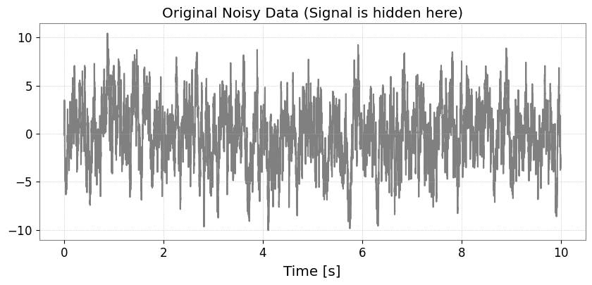
Step 1: Generating Colored Noise and Injecting a Signal

First, we create colored noise with strong low-frequency components (AR(1) process), and embed a weak signal (sine-Gaussian) that is difficult to distinguish otherwise. Note: We use “strain” as the unit, which is recognizable by Astropy.

import matplotlib.pyplot as plt
import numpy as np

from gwexpy.timeseries import TimeSeries


def generate_mock_data(duration=10, fs=1024):
    t = np.linspace(0, duration, int(duration * fs))

    # 1. Background Noise (AR(1) process with strong autocorrelation)
    np.random.seed(42)
    white_noise = np.random.normal(0, 1, len(t))
    colored_noise = np.zeros_like(white_noise)
    for i in range(1, len(t)):
        colored_noise[i] = 0.95 * colored_noise[i - 1] + white_noise[i]

    # 2. Injected Signal (Sine-Gaussian)
    center_time = 5.0
    sig_freq = 50.0
    width = 0.1
    signal = (
        2.0
        * np.exp(-((t - center_time) ** 2) / (2 * width**2))
        * np.sin(2 * np.pi * sig_freq * t)
    )

    data = colored_noise + signal
    # Use a standard unit string that astropy/gwpy can recognize
    return TimeSeries(data, t0=0, dt=1 / fs, unit="strain", name="MockData")


ts = generate_mock_data()

plt.figure(figsize=(10, 4))
plt.plot(ts, color="gray")
plt.title("Original Noisy Data (Signal is hidden here)")
plt.xlabel("Time [s]")
plt.grid(True, linestyle=":")
plt.show()

Step 2: Noise Modeling with ARIMA

Using auto=True, we search for the optimal model that expresses the autocorrelation structure of the background noise.

print("Searching for optimal noise model parameters...")
# We prioritize AR model for whitening, so we set max_p=5 and max_q=0.
model = ts.arima(auto=True, max_p=5, max_q=0)
print(f"Best model order: {model.res.model.order}")
print(model.summary())

Searching for optimal noise model parameters...
Best model order: (5, 1, 0)
                               SARIMAX Results
==============================================================================
Dep. Variable:                      y   No. Observations:                10240
Model:               SARIMAX(5, 1, 0)   Log Likelihood              -14694.968
Date:                Thu, 26 Feb 2026   AIC                          29403.936
Time:                        20:48:38   BIC                          29454.574
Sample:                             0   HQIC                         29421.057
                              - 10240
Covariance Type:                  opg
==============================================================================
                 coef    std err          z      P>|z|      [0.025      0.975]
------------------------------------------------------------------------------
intercept     -0.0003      0.010     -0.033      0.973      -0.020       0.019
ar.L1         -0.0379      0.010     -3.794      0.000      -0.057      -0.018
ar.L2         -0.0413      0.010     -4.150      0.000      -0.061      -0.022
ar.L3         -0.0271      0.010     -2.692      0.007      -0.047      -0.007
ar.L4         -0.0303      0.010     -3.078      0.002      -0.050      -0.011
ar.L5         -0.0216      0.010     -2.195      0.028      -0.041      -0.002
sigma2         1.0330      0.014     72.089      0.000       1.005       1.061
===================================================================================
Ljung-Box (L1) (Q):                   0.01   Jarque-Bera (JB):                 0.54
Prob(Q):                              0.94   Prob(JB):                         0.76
Heteroskedasticity (H):               1.03   Skew:                             0.01
Prob(H) (two-sided):                  0.35   Kurtosis:                         3.03
===================================================================================

Warnings:
[1] Covariance matrix calculated using the outer product of gradients (complex-step).

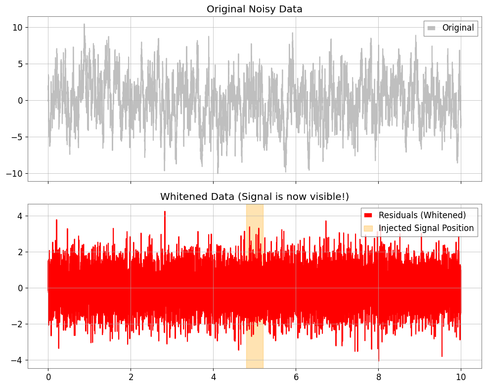
Step 3: Extracting and Visualizing Residuals

By subtracting the “stationary noise” predicted by the model, we obtain the residuals \(x_r = x - \hat{x}\). This is the whitened data.

ts_whitened = model.residuals()
ts_whitened.name = "Whitened Data"

fig, ax = plt.subplots(2, 1, figsize=(10, 8), sharex=True)

ax[0].plot(ts, color="gray", alpha=0.5, label="Original")
ax[0].set_title("Original Noisy Data")
ax[0].legend(loc="upper right")

ax[1].plot(ts_whitened, color="red", label="Residuals (Whitened)")
ax[1].set_title("Whitened Data (Signal is now visible!)")
ax[1].axvspan(4.8, 5.2, color="orange", alpha=0.3, label="Injected Signal Position")
ax[1].legend(loc="upper right")

plt.tight_layout()
plt.show()

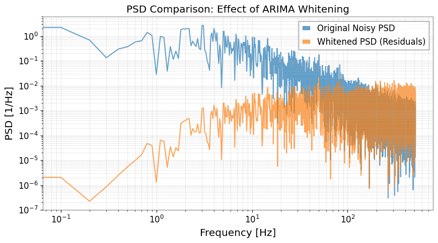
Step 4: Evaluation in the Frequency Domain

We calculate and compare the Power Spectral Density (PSD).

fft_original = ts.psd()
fft_whitened = ts_whitened.psd()

plt.figure(figsize=(10, 5))
plt.loglog(
    fft_original.frequencies.value,
    fft_original.value,
    label="Original Noisy PSD",
    alpha=0.7,
)
plt.loglog(
    fft_whitened.frequencies.value,
    fft_whitened.value,
    label="Whitened PSD (Residuals)",
    alpha=0.7,
)
plt.title("PSD Comparison: Effect of ARIMA Whitening")
plt.xlabel("Frequency [Hz]")
plt.ylabel("PSD [1/Hz]")
plt.legend()
plt.grid(True, which="both", linestyle=":")
plt.show()

Summary

• Using model.residuals(), whitening can be easily performed without writing complex mathematical formulas.

• This technique is very powerful for searching for burst signals in gravitational wave analysis and for extracting ringdown waveforms (exponentially decaying sinusoids) immediately after events.