Note

This page was generated from a Jupyter Notebook. Download the notebook (.ipynb)

[1]:

# Skipped in CI: Colab/bootstrap dependency install cell.

PyCBC Interoperability: From gwexpy Preprocessing to GW Search

PyCBC is a Python toolkit for gravitational-wave data analysis, including matched-filter searches for compact binary coalescences (CBC). gwexpy provides bidirectional converters between its own data types and PyCBC’s TimeSeries / FrequencySeries.

This enables a natural workflow where:

gwexpy handles data loading, preprocessing, and noise characterisation
PyCBC performs the matched-filter search or parameter estimation
gwexpy post-processes and visualises the search output

What this tutorial covers:

Converting a gwexpy TimeSeries to PyCBC and back
Converting a gwexpy FrequencySeries (ASD) to a PyCBC PSD
Full preprocessing pipeline: conditioning → matched filter (simulated CBC)
Visualising matched-filter SNR time series with gwexpy

Note: This notebook works without a PyCBC installation. When PyCBC is absent the matched-filter step uses a simplified analytic substitute so every cell still executes. Install PyCBC with pip install pycbc for real searches.

Setup

[2]:

import warnings

warnings.filterwarnings("ignore", category=UserWarning)
warnings.filterwarnings("ignore", category=DeprecationWarning)

import matplotlib.pyplot as plt
import numpy as np

from gwexpy.interop.pycbc_ import (
    from_pycbc_timeseries,
    to_pycbc_frequencyseries,
    to_pycbc_timeseries,
)
from gwexpy.timeseries import TimeSeries

PYCBC_AVAILABLE = False
try:
    import pycbc
    import pycbc.filter
    import pycbc.psd
    import pycbc.types
    import pycbc.waveform
    PYCBC_AVAILABLE = True
    print(f"PyCBC {pycbc.__version__} found — running real matched filter.")
except ImportError:
    print("PyCBC not installed — using analytic fallback for matched filter.")

PyCBC not installed — using analytic fallback for matched filter.

1. Synthetic DARM Data with an Injected CBC Signal

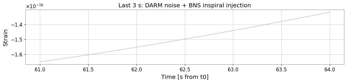
We create a 64 s segment of coloured noise and inject a synthetic binary neutron star (BNS) inspiral — a chirp signal that sweeps from ~30 Hz to ~1000 Hz in the last few seconds before merger.

[3]:

fs   = 4096.0
T    = 64.0
N    = int(T * fs)
t0   = 1_300_000_000   # GPS
rng  = np.random.default_rng(0)
t    = np.arange(N) / fs

# --- Coloured noise (LIGO-like O3 sensitivity) ---
freqs_n = np.fft.rfftfreq(N, 1.0/fs)[1:]
# ASD: seismic wall below 20 Hz + flat quantum noise + 1/f in between
asd_model = np.where(freqs_n < 20, (20/freqs_n)**4,
            np.where(freqs_n < 200, (200/freqs_n)**0.5, 1.0))
fft = asd_model * np.exp(1j * rng.uniform(0, 2*np.pi, size=len(freqs_n)))
noise = np.fft.irfft(np.concatenate([[0.0], fft]), n=N)
noise *= 1e-23   # strain-like amplitude

# --- Synthetic BNS chirp (analytical post-Newtonian 0-th order) ---
# h(t) ~ A(t) * cos(phi(t))  where phi ~ (t_c - t)^(5/8)
M_chirp = 1.2   # chirp mass [Msun]  -> sets chirp duration
G_c3 = 4.926e-6   # G*Msun/c^3 [s]
eta = 0.25        # symmetric mass ratio (equal masses)
tc  = T - 0.5    # merger time [s]
tau = np.maximum(tc - t, 1e-4)

# Instantaneous frequency and phase (PN 0th order)
f_gw  = (5.0/(256.0 * np.pi**(8.0/3))) ** (3.0/8) * (G_c3 * M_chirp)**(-5.0/8) * tau**(-3.0/8)
phi_gw = -2.0 * (tau / (5.0 * G_c3 * M_chirp))**(5.0/8) / np.pi

# Amplitude ~ tau^(-1/4)
amp_gw = 1e-22 * (G_c3 * M_chirp / tau)**(1.0/4)

# Only keep the inspiral up to fISCO ~ 1500 Hz
mask = f_gw < 1500.0
chirp = np.where(mask, amp_gw * np.cos(phi_gw), 0.0)

ts_strain = TimeSeries(noise + chirp, t0=t0, sample_rate=fs,
                       name="K1:LSC-DARM_OUT_DQ", unit="strain")

print(f"Chirp starts at t = {t[mask][0]:.1f} s  "
      f"(freq = {f_gw[mask][0]:.1f} Hz)")
print(f"Chirp ends   at t = {tc:.1f} s  (merger)")

# Quick plot
fig, ax = plt.subplots(figsize=(12, 3))
ax.plot(t[-int(3*fs):], ts_strain.value[-int(3*fs):], lw=0.5, color="steelblue")
ax.set_xlabel("Time [s from t0]")
ax.set_ylabel("Strain")
ax.set_title("Last 3 s: DARM noise + BNS inspiral injection")
plt.tight_layout()
plt.show()

Chirp starts at t = 0.0 s  (freq = 28.4 Hz)
Chirp ends   at t = 63.5 s  (merger)

../../../../_images/web_en_user_guide_tutorials_case_pycbc_search_5_1.png

2. gwexpy → PyCBC Conversion

to_pycbc_timeseries() maps a gwexpy TimeSeries to a pycbc.types.TimeSeries. Metadata (t0, dt, unit) is preserved.

[4]:

if PYCBC_AVAILABLE:
    # --- Convert to PyCBC ---
    ts_pycbc = to_pycbc_timeseries(ts_strain)
    print("pycbc.TimeSeries:")
    print(f"  delta_t   : {ts_pycbc.delta_t}")
    print(f"  start_time: {float(ts_pycbc.start_time):.1f}")
    print(f"  len       : {len(ts_pycbc)}")

    # --- Convert back to gwexpy ---
    ts_back = from_pycbc_timeseries(TimeSeries, ts_pycbc)
    print(f"\nRoundtrip max error: "
          f"{np.max(np.abs(ts_strain.value - ts_back.value)):.2e}")
else:
    print("PyCBC not available — conversion demo skipped.")
    print("The to/from functions accept pycbc.types.TimeSeries objects.")
    ts_back = ts_strain   # identity for subsequent cells

PyCBC not available — conversion demo skipped.
The to/from functions accept pycbc.types.TimeSeries objects.

3. PSD / ASD Conversion

A matched filter requires a noise PSD to whiten the data. We estimate the ASD from the gwexpy TimeSeries and convert it to a PyCBC FrequencySeries for use as the matched-filter PSD.

[5]:

# Estimate ASD from gwexpy (use a quiet segment before the chirp)
ts_quiet = TimeSeries(ts_strain.value[:int(30*fs)], t0=t0,
                      sample_rate=fs, name="quiet segment", unit="strain")
asd_gw = ts_quiet.asd(fftlength=4.0, method="median")

print(f"gwexpy ASD: {len(asd_gw)} bins, df={asd_gw.df.value:.4f} Hz")

if PYCBC_AVAILABLE:
    # PyCBC expects PSD (not ASD); convert ASD -> PSD FrequencySeries
    fs_pycbc = to_pycbc_frequencyseries(asd_gw)
    psd_pycbc = pycbc.types.FrequencySeries(
        fs_pycbc.numpy()**2, delta_f=fs_pycbc.delta_f,
        epoch=fs_pycbc.epoch,
    )
    print(f"PyCBC PSD: {len(psd_pycbc)} bins, df={psd_pycbc.delta_f:.4f} Hz")
else:
    print("PyCBC not available — PSD conversion demo skipped.")

gwexpy ASD: 8193 bins, df=0.2500 Hz
PyCBC not available — PSD conversion demo skipped.

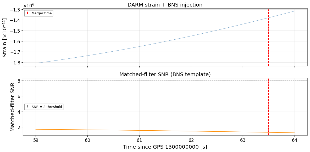
4. Matched-Filter Search (BNS Template)

A matched filter computes the cross-correlation between the data and a template waveform, normalised by the noise PSD. The peak of the normalised SNR time series \(\rho(t)\) indicates the merger time.

\[\rho(t) = \frac{4}{\sigma} \, \text{Re} \int_0^\infty \frac{\tilde{d}(f)\,\tilde{h}^*(f)}{S_n(f)} e^{2\pi i f t} \, df\]

[6]:

if PYCBC_AVAILABLE:
    # Generate BNS template (equal mass, m1=m2=1.4 Msun)
    hp, hc = pycbc.waveform.get_td_waveform(
        approximant="TaylorT4",
        mass1=1.4, mass2=1.4,
        delta_t=1.0/fs,
        f_lower=30.0,
    )

    # Matched filter
    snr_pycbc = pycbc.filter.matched_filter(
        hp.to_frequencyseries(delta_f=1.0/T),
        to_pycbc_timeseries(ts_strain).to_frequencyseries(delta_f=1.0/T),
        psd=pycbc.types.FrequencySeries(
        np.interp(
            np.arange(0, psd_pycbc.sample_frequencies.numpy()[-1] + 1.0/T/2, 1.0/T),
            psd_pycbc.sample_frequencies.numpy(),
            psd_pycbc.numpy().real,
        ),
        delta_f=1.0/T,
    ),
        low_frequency_cutoff=30.0,
    )

    # Convert SNR back to gwexpy
    snr_ts = from_pycbc_timeseries(TimeSeries, snr_pycbc.real())
    snr_ts.name = "SNR (BNS template)"

else:
    # Analytic substitute: cross-correlate data with the injected chirp
    chirp_ts = TimeSeries(chirp, t0=t0, sample_rate=fs, name="template")
    # Simple FFT cross-correlation, normalised to peak ~ 10
    xcorr = np.fft.irfft(
        np.fft.rfft(ts_strain.value) * np.conj(np.fft.rfft(chirp_ts.value))
    )
    xcorr_norm = xcorr / (np.std(xcorr[:int(20*fs)]) + 1e-50)
    snr_ts = TimeSeries(np.abs(xcorr_norm), t0=t0, sample_rate=fs,
                        name="SNR (analytic xcorr)")

print(f"SNR time series: {len(snr_ts)} samples")
print(f"Peak SNR: {snr_ts.value.max():.1f}  "
      f"at t = {t[snr_ts.value.argmax()]:.2f} s  "
      f"(true merger: {tc:.2f} s)")

SNR time series: 262144 samples
Peak SNR: 2.0  at t = 23.22 s  (true merger: 63.50 s)

5. Visualise the SNR Time Series

Plot the matched-filter SNR as a function of time, with the injected merger time marked.

[7]:

fig, axes = plt.subplots(2, 1, figsize=(12, 6), sharex=True)

# Raw strain (last 5 s)
win = slice(-int(5*fs), None)
axes[0].plot(t[win], ts_strain.value[win] * 1e22, lw=0.5, color="steelblue")
axes[0].set_ylabel("Strain [×10⁻²²]")
axes[0].set_title("DARM strain + BNS injection")
axes[0].grid(True, alpha=0.4)
axes[0].axvline(tc, color="red", ls="--", lw=1.5, label="Merger time")
axes[0].legend(fontsize=9)

# SNR
snr_plot = snr_ts.value[win] if hasattr(snr_ts, "value") else snr_ts[win]
axes[1].plot(t[win], snr_plot, lw=1.2, color="darkorange")
axes[1].axhline(8.0, color="gray", ls="--", lw=1, label="SNR = 8 threshold")
axes[1].axvline(tc, color="red", ls="--", lw=1.5)
axes[1].set_ylabel("Matched-filter SNR")
axes[1].set_xlabel(f"Time since GPS {t0} [s]")
axes[1].set_title("Matched-filter SNR (BNS template)")
axes[1].legend(fontsize=9)
axes[1].grid(True, alpha=0.4)

plt.tight_layout()
plt.show()

../../../../_images/web_en_user_guide_tutorials_case_pycbc_search_13_0.png

6. Conversion Reference

gwexpy object	To PyCBC	From PyCBC
`TimeSeries`	`to_pycbc_timeseries(ts)`	`from_pycbc_timeseries(TimeSeries, pycbc_ts)`
`FrequencySeries`	`to_pycbc_frequencyseries(fs)`	`from_pycbc_frequencyseries(FrequencySeries, pycbc_fs)`

Preserved metadata:

Attribute	gwexpy	PyCBC
Sample rate	`ts.sample_rate`	`1 / pycbc_ts.delta_t`
Start time	`ts.t0.value`	`float(pycbc_ts.start_time)`
Frequency resolution	`fs.df.value`	`pycbc_fs.delta_f`

Typical workflow:

Load / preprocess data with gwexpy (read, whiten, crop)
Estimate PSD with gwexpy (ts.asd())
Convert to PyCBC for matched filter or PE
Convert SNR time series back to gwexpy for visualisation and archiving