Note

This page was generated from a Jupyter Notebook. Download the notebook (.ipynb)

Introduction to ScalarField Class

This notebook teaches the basic usage of the ScalarField class in gwexpy.

What is ScalarField?

ScalarField is a specialized class for handling 4-dimensional data consisting of time and 3D space. It represents the spacetime structure of physical fields and provides the following features:

• Axis 0 (time axis): Time domain ↔ Frequency domain transformations

• Axes 1-3 (spatial axes): Real space ↔ K-space (wavenumber space) transformations

• 4D structure preservation: Always maintains 4 dimensions even when sliced

• Batch operations: Bulk processing of multiple fields using FieldList and FieldDict

• Signal processing: PSD calculation, frequency-space mapping, cross-correlation, coherence maps

Setup

Import the necessary libraries.

# Suppress SWIGLAL and other warnings for clean output
import warnings

warnings.filterwarnings("ignore", "Wswiglal-redir-stdio")
warnings.filterwarnings("ignore", category=UserWarning)

# Helper functions for visualization
def show_field_info(field, title="Field Information"):
    """Display field metadata as a formatted table"""
    import pandas as pd
    from IPython.display import HTML, display

    info = {
        'Property': ['Shape', 'Time Domain', 'Space Domains', 'Axis 0', 'Axis 1', 'Axis 2', 'Axis 3'],
        'Value': [
            str(field.shape),
            field.time_domain,
            str(field.space_domains),
            f"{field.axis0_name} ({field.shape[0]} points)",
            f"{field.axis1_name} ({field.shape[1]} points)",
            f"{field.axis2_name} ({field.shape[2]} points)",
            f"{field.axis3_name} ({field.shape[3]} points)"
        ]
    }
    df = pd.DataFrame(info)
    display(HTML(f"<h4>{title}</h4>"))
    display(df.to_html(index=False, border=1))

def compare_fields(field1, field2, name1="Original", name2="Processed"):
    """Compare two fields side by side"""
    import pandas as pd
    from IPython.display import HTML, display

    comparison = {
        'Property': ['Shape', 'Time Domain', 'Space Domains', 'Max Difference'],
        name1: [
            str(field1.shape),
            field1.time_domain,
            str(field1.space_domains),
            'N/A'
        ],
        name2: [
            str(field2.shape),
            field2.time_domain,
            str(field2.space_domains),
            f"{np.max(np.abs(field1.value - field2.value)):.2e}"
        ]
    }
    df = pd.DataFrame(comparison)
    display(HTML("<h4>Field Comparison</h4>"))
    display(df.to_html(index=False, border=1))

import matplotlib.pyplot as plt
import numpy as np
from astropy import units as u

from gwexpy.fields import FieldDict, FieldList, ScalarField

# Set seed for reproducibility
np.random.seed(42)

1. ScalarField Initialization and Metadata

Create a ScalarField object and check its metadata.

# Create 4D data (10 time points × 8×8×8 spatial grid)
nt, nx, ny, nz = 10, 8, 8, 8
data = np.random.randn(nt, nx, ny, nz)

# Define axis coordinates
t = np.arange(nt) * 0.1 * u.s
x = np.arange(nx) * 0.5 * u.m
y = np.arange(ny) * 0.5 * u.m
z = np.arange(nz) * 0.5 * u.m

# Create ScalarField object
field = ScalarField(
    data,
    unit=u.V,
    axis0=t,
    axis1=x,
    axis2=y,
    axis3=z,
    axis_names=["t", "x", "y", "z"],
    axis0_domain="time",
    space_domain="real",
)

print(f"Shape: {field.shape}")
print(f"Unit: {field.unit}")
print(f"Axis names: {field.axis_names}")
print(f"Axis0 domain: {field.axis0_domain}")
print(f"Space domains: {field.space_domains}")

Shape: (10, 8, 8, 8)
Unit: V
Axis names: ('t', 'x', 'y', 'z')
Axis0 domain: time
Space domains: {'x': 'real', 'y': 'real', 'z': 'real'}

Checking Metadata

• axis0_domain: Domain of axis 0 (“time” or “frequency”)

• space_domains: Domain of each spatial axis (“real” or “k”)

• axis_names: Name of each axis

These metadata are automatically updated during FFT transformations.

2. Slicing with 4D Structure Preservation

An important feature of ScalarField is that it always maintains 4 dimensions even when sliced. Even when using integer indices, they are automatically converted to length-1 slices.

# Slice with integer index (would become 3D with regular ndarray)
sliced = field[0, :, :, :]

print(f"Original shape: {field.shape}")
print(f"Sliced shape: {sliced.shape}")  # (1, 8, 8, 8) - maintains 4D!
print(f"Type: {type(sliced)}")  # Still a ScalarField
print(f"Axis names preserved: {sliced.axis_names}")

Original shape: (10, 8, 8, 8)
Sliced shape: (1, 8, 8, 8)
Type: <class 'gwexpy.fields.scalar.ScalarField'>
Axis names preserved: ('t', 'x', 'y', 'z')

# Use integer indices on multiple axes
sliced_multi = field[0, 1, 2, 3]

print(f"Multi-sliced shape: {sliced_multi.shape}")  # (1, 1, 1, 1) - still 4D
print(f"Value: {sliced_multi.value}")

Multi-sliced shape: (1, 1, 1, 1)
Value: [[[[-0.51827022]]]]

This behavior maintains the consistency of ScalarField objects, and metadata (axis names and domain information) are never lost.

3. Time-Frequency Transformation (FFT on Axis 0)

You can transform the time axis to the frequency axis using the fft_time() and ifft_time() methods. The same normalization as GWpy’s TimeSeries.fft() is adopted.

# Create ScalarField in time domain (sine wave)
t_dense = np.arange(128) * 0.01 * u.s
x_small = np.arange(4) * 1.0 * u.m
signal_freq = 10.0  # Hz

# Place a 10 Hz sine wave uniformly in space
data_signal = np.sin(2 * np.pi * signal_freq * t_dense.value)[:, None, None, None]
data_signal = np.tile(data_signal, (1, 4, 4, 4))

field_time = ScalarField(
    data_signal,
    unit=u.V,
    axis0=t_dense,
    axis1=x_small,
    axis2=x_small.copy(),
    axis3=x_small.copy(),
    axis_names=["t", "x", "y", "z"],
    axis0_domain="time",
    space_domain="real",
)

# Execute FFT
field_freq = field_time.fft_time()

print(f"Time domain shape: {field_time.shape}")
print(f"Frequency domain shape: {field_freq.shape}")
print(f"Axis0 domain changed: {field_time.axis0_domain} → {field_freq.axis0_domain}")

Time domain shape: (128, 4, 4, 4)
Frequency domain shape: (65, 4, 4, 4)
Axis0 domain changed: time → frequency

# Plot frequency spectrum (select one point in x,y,z)
# Note: Since 4D structure is maintained even after slicing, squeeze() is used to reduce dimensions
spectrum = np.abs(field_freq[:, 0, 0, 0].value).squeeze()
freqs = field_freq._axis0_index.value

plt.figure(figsize=(10, 4))
plt.plot(freqs, spectrum, "b-", linewidth=2)
plt.axvline(
    signal_freq, color="r", linestyle="--", label=f"{signal_freq} Hz (Input signal)"
)
plt.xlabel("Frequency [Hz]")
plt.ylabel("Amplitude [V]")
plt.title("FFT Spectrum (ScalarField)")
plt.xlim(0, 50)
plt.legend()
plt.grid(True, alpha=0.3)
plt.tight_layout()
plt.show()

# Check peak frequency
peak_idx = np.argmax(spectrum)
peak_freq = freqs[peak_idx]
print(f"Peak frequency: {peak_freq:.2f} Hz (expected: {signal_freq} Hz)")

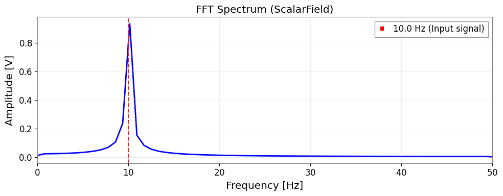
Peak frequency: 10.16 Hz (expected: 10.0 Hz)

Inverse FFT (Frequency → Time)

You can return to the original time domain with ifft_time().

# Inverse FFT
field_reconstructed = field_freq.ifft_time()

# Compare with original signal
# Note: squeeze() to 1D to maintain 4D structure
original = field_time[:, 0, 0, 0].value.squeeze()
reconstructed = field_reconstructed[:, 0, 0, 0].value.squeeze()

plt.figure(figsize=(10, 4))
plt.plot(t_dense.value, original, "b-", label="Original", alpha=0.7)
plt.plot(t_dense.value, reconstructed.real, "r--", label="Reconstructed", alpha=0.7)
plt.xlabel("Time [s]")
plt.ylabel("Amplitude [V]")
plt.title("IFFT: Frequency → Time")
plt.legend()
plt.grid(True, alpha=0.3)
plt.tight_layout()
plt.show()

# Check error
error = np.abs(original - reconstructed.real)
print(f"Max reconstruction error: {np.max(error):.2e} V")

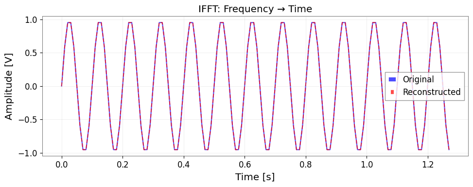
Max reconstruction error: 4.44e-16 V

4. Real Space-K Space Transformation (FFT on Spatial Axes)

You can transform spatial axes to wavenumber space (K-space) using fft_space() and ifft_space(). Signed FFT with angular wavenumber k = 2π / λ is used.

# Create data with periodic structure in space
nx, ny, nz = 16, 16, 16
x_grid = np.arange(nx) * 0.5 * u.m
y_grid = np.arange(ny) * 0.5 * u.m
z_grid = np.arange(nz) * 0.5 * u.m

# Sine wave with wavelength 4m in X direction
wavelength = 4.0  # m
k_expected = 2 * np.pi / wavelength  # rad/m

data_spatial = np.sin(2 * np.pi * x_grid.value / wavelength)[None, :, None, None]
data_spatial = np.tile(data_spatial, (4, 1, ny, nz))

field_real = ScalarField(
    data_spatial,
    unit=u.V,
    axis0=np.arange(4) * 0.1 * u.s,
    axis1=x_grid,
    axis2=y_grid,
    axis3=z_grid,
    axis_names=["t", "x", "y", "z"],
    axis0_domain="time",
    space_domain="real",
)

# FFT only on X axis
field_kx = field_real.fft_space(axes=["x"])

print(f"Original space domains: {field_real.space_domains}")
print(f"After fft_space: {field_kx.space_domains}")
print(f"Axis names: {field_kx.axis_names}")

Original space domains: {'x': 'real', 'y': 'real', 'z': 'real'}
After fft_space: {'y': 'real', 'z': 'real', 'kx': 'k'}
Axis names: ('t', 'kx', 'y', 'z')

# Plot K-space spectrum
# Note: squeeze() to reduce dimensions
kx_spectrum = np.abs(field_kx[0, :, 0, 0].value).squeeze()
kx_values = field_kx._axis1_index.value

plt.figure(figsize=(10, 4))
plt.plot(kx_values, kx_spectrum, "b-", linewidth=2)
plt.axvline(k_expected, color="r", linestyle="--", label=f"k = {k_expected:.2f} rad/m")
plt.axvline(-k_expected, color="r", linestyle="--")
plt.xlabel("Wavenumber kx [rad/m]")
plt.ylabel("Amplitude")
plt.title("Spatial FFT: Real → K space")
plt.legend()
plt.grid(True, alpha=0.3)
plt.tight_layout()
plt.show()

# Check peak wavenumber
peak_idx = np.argmax(kx_spectrum)
peak_k = kx_values[peak_idx]
print(f"Peak wavenumber: {peak_k:.2f} rad/m (expected: ±{k_expected:.2f} rad/m)")

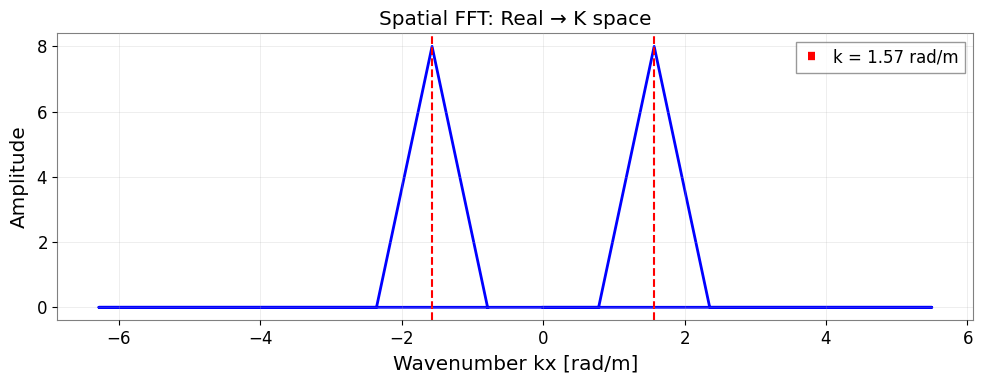
Peak wavenumber: 1.57 rad/m (expected: ±1.57 rad/m)

Wavelength Calculation

In K-space, you can calculate the wavelength using the wavelength() method.

# Calculate wavelength
wavelengths = field_kx.wavelength("kx")

print(f"Wavelength at k={k_expected:.2f}: {2 * np.pi / k_expected:.2f} m")
print(
    f"Calculated wavelengths range: {wavelengths.value[wavelengths.value > 0].min():.2f} - {wavelengths.value[wavelengths.value < np.inf].max():.2f} m"
)

Wavelength at k=1.57: 4.00 m
Calculated wavelengths range: 1.00 - 8.00 m

FFT on All Spatial Axes

If you omit the axes parameter, you can FFT all spatial axes together.

# FFT on all spatial axes
field_k_all = field_real.fft_space()
print(f"All spatial axes in K space: {field_k_all.space_domains}")

# Return to original with inverse FFT
field_real_back = field_k_all.ifft_space()
print(f"Back to real space: {field_real_back.space_domains}")

# Reconstruction error
reconstruction_error = np.max(np.abs(field_real.value - field_real_back.value))
print(f"Max reconstruction error: {reconstruction_error:.2e}")

All spatial axes in K space: {'kx': 'k', 'ky': 'k', 'kz': 'k'}
Back to real space: {'x': 'real', 'y': 'real', 'z': 'real'}
Max reconstruction error: 2.29e-16

5. Batch Operations with FieldList and FieldDict

To process multiple ScalarField objects together, use FieldList or FieldDict.

FieldList

Manage multiple fields in list format and apply FFT operations in bulk.

# Create three ScalarFields with different amplitudes
amplitudes = [1.0, 2.0, 3.0]
fields = []

for amp in amplitudes:
    data_temp = amp * np.random.randn(8, 4, 4, 4)
    field_temp = ScalarField(
        data_temp,
        unit=u.V,
        axis0=np.arange(8) * 0.1 * u.s,
        axis1=np.arange(4) * 0.5 * u.m,
        axis2=np.arange(4) * 0.5 * u.m,
        axis3=np.arange(4) * 0.5 * u.m,
        axis_names=["t", "x", "y", "z"],
        axis0_domain="time",
        space_domain="real",
    )
    fields.append(field_temp)

# Create FieldList
field_list = FieldList(fields, validate=True)
print(f"Number of fields: {len(field_list)}")

Number of fields: 3

# Execute time FFT in bulk
field_list_freq = field_list.fft_time_all()

print("All fields transformed to frequency domain:")
for i, field in enumerate(field_list_freq):
    print(f"  Field {i}: axis0_domain = {field.axis0_domain}")

All fields transformed to frequency domain:
  Field 0: axis0_domain = frequency
  Field 1: axis0_domain = frequency
  Field 2: axis0_domain = frequency

FieldDict

Manage named fields in dictionary format.

# Create dictionary of named fields
field_dict = FieldDict(
    {"channel_A": fields[0], "channel_B": fields[1], "channel_C": fields[2]},
    validate=True,
)

print(f"Field names: {list(field_dict.keys())}")

Field names: ['channel_A', 'channel_B', 'channel_C']

# Execute spatial FFT in bulk
field_dict_k = field_dict.fft_space_all(axes=["x", "y"])

for name, field in field_dict_k.items():
    print(f"{name}: {field.space_domains}")

channel_A: {'z': 'real', 'kx': 'k', 'ky': 'k'}
channel_B: {'z': 'real', 'kx': 'k', 'ky': 'k'}
channel_C: {'z': 'real', 'kx': 'k', 'ky': 'k'}

6. Signal Processing and Analysis

As important signal processing techniques for physical field analysis, we demonstrate the following:

1. PSD calculation: Power spectral density in time and spatial directions

2. Frequency-space mapping: Visualize how frequency changes spatially

3. Cross-correlation: Estimate signal propagation delays

4. Coherence map: Visualize spatial coherence

# Generate simulation data
# Signal: 30 Hz sine wave propagating from x=1m
# Noise: Gaussian noise
fs = 256 * u.Hz
duration = 4 * u.s
t = np.arange(int((fs * duration).to_value(u.dimensionless_unscaled))) / fs.value
x = np.linspace(0, 5, 20)  # 5m, 20 points
y = np.linspace(0, 2, 5)  # 2m, 5 points
z = np.array([0])  # z=0

shape = (len(t), len(x), len(y), len(z))
data_sig = np.random.normal(0, 0.1, size=shape)

source_freq = 30.0
source_signal = np.sin(2 * np.pi * source_freq * t)
v_prop = 10.0  # 10 m/s
source_pos = 1.0

for i, xi in enumerate(x):
    dist = abs(xi - source_pos)
    delay = dist / v_prop
    shift = int(delay * fs.value)
    sig_delayed = np.roll(source_signal, shift)
    amp = 1.0 / (1.0 + dist)
    data_sig[:, i, :, 0] += amp * sig_delayed[:, np.newaxis]

field_sig = ScalarField(
    data_sig,
    unit=u.V,
    axis0=t * u.s,
    axis1=x * u.m,
    axis2=y * u.m,
    axis3=z * u.m,
    name="Environmental Field",
)
print(field_sig)

ScalarField([[[[ 0.08684844],
               [ 0.36739322],
               [ 0.20264566],
               [ 0.24368612],
               [ 0.29709332]],

              [[-0.42828167],
               [-0.2788319 ],
               [-0.63601112],
               [-0.43725569],
               [-0.45766302]],

              [[-0.50234469],
               [-0.39848957],
               [-0.33841909],
               [-0.30672809],
               [-0.35290641]],

              ...,

              [[-0.24582327],
               [-0.36331307],
               [-0.35576048],
               [-0.30664571],
               [-0.29873314]],

              [[-0.25188483],
               [-0.10460112],
               [-0.20704192],
               [-0.17437447],
               [-0.06699974]],

              [[-0.01857532],
               [ 0.03160235],
               [ 0.09463293],
               [-0.13609984],
               [-0.18043362]]],


             [[[ 0.4965515 ],
               [ 0.51114119],
               [ 0.66836178],
               [ 0.47774925],
               [ 0.54391374]],

              [[ 0.00870382],
               [ 0.05797381],
               [ 0.19497677],
               [-0.1841482 ],
               [ 0.06961271]],

              [[-0.44467682],
               [-0.63003207],
               [-0.4931782 ],
               [-0.72115671],
               [-0.66144024]],

              ...,

              [[-0.26696884],
               [-0.02335534],
               [-0.2955512 ],
               [ 0.03365938],
               [-0.16675011]],

              [[-0.01148699],
               [ 0.02693153],
               [ 0.23230027],
               [-0.12005181],
               [-0.1327343 ]],

              [[ 0.0960591 ],
               [ 0.17476004],
               [-0.00103139],
               [ 0.17377965],
               [ 0.34090044]]],


             [[[ 0.48591277],
               [ 0.44150349],
               [ 0.40895599],
               [ 0.5606232 ],
               [ 0.38818876]],

              [[ 0.59176168],
               [ 0.60045806],
               [ 0.43279717],
               [ 0.40597058],
               [ 0.51018807]],

              [[-0.48896672],
               [-0.67904575],
               [-0.65110209],
               [-0.73068132],
               [-0.55754008]],

              ...,

              [[-0.00889405],
               [ 0.0246277 ],
               [-0.00934052],
               [-0.28479022],
               [ 0.00294349]],

              [[-0.05809312],
               [ 0.21557047],
               [ 0.08898029],
               [ 0.19601207],
               [-0.00748609]],

              [[ 0.31327382],
               [ 0.04965958],
               [ 0.12931156],
               [ 0.09634759],
               [ 0.02072857]]],


             ...,


             [[[-0.47088405],
               [-0.44093954],
               [-0.50808846],
               [-0.53825154],
               [-0.52270623]],

              [[-0.27016794],
               [-0.05885403],
               [-0.03014553],
               [-0.11945106],
               [-0.22574645]],

              [[ 0.67186813],
               [ 0.65758934],
               [ 0.61808806],
               [ 0.68006628],
               [ 0.64916691]],

              ...,

              [[ 0.33427533],
               [ 0.1238872 ],
               [ 0.23921193],
               [ 0.13288922],
               [ 0.17767688]],

              [[-0.09293398],
               [ 0.04599217],
               [-0.04333049],
               [-0.14249861],
               [-0.14613857]],

              [[-0.17523055],
               [-0.08070457],
               [-0.3736138 ],
               [-0.21547623],
               [-0.24905171]]],


             [[[-0.33979978],
               [-0.52516958],
               [-0.43117016],
               [-0.55575497],
               [-0.30922288]],

              [[-0.57172495],
               [-0.36253384],
               [-0.47323134],
               [-0.56822764],
               [-0.41788518]],

              [[ 0.60000133],
               [ 0.69520425],
               [ 0.58067915],
               [ 0.59044121],
               [ 0.60903589]],

              ...,

              [[ 0.09738152],
               [-0.03127321],
               [ 0.10558964],
               [ 0.02092155],
               [ 0.12403775]],

              [[-0.17854237],
               [-0.15159656],
               [-0.13889632],
               [-0.10361625],
               [-0.07109176]],

              [[-0.30326966],
               [-0.18659539],
               [-0.17075845],
               [ 0.12720352],
               [-0.09463939]]],


             [[[-0.13293935],
               [-0.26827271],
               [-0.16340608],
               [ 0.0859768 ],
               [-0.29470039]],

              [[-0.59042514],
               [-0.43746394],
               [-0.34756977],
               [-0.58880771],
               [-0.50722801]],

              [[ 0.19803234],
               [ 0.1693735 ],
               [ 0.13092929],
               [ 0.23941187],
               [ 0.22039804]],

              ...,

              [[-0.17123032],
               [-0.04474158],
               [-0.08665946],
               [-0.00431457],
               [-0.00958998]],

              [[-0.12704775],
               [-0.18034525],
               [-0.24545939],
               [-0.26021225],
               [-0.27972791]],

              [[-0.10539607],
               [ 0.00241909],
               [ 0.01135068],
               [-0.2382848 ],
               [-0.06614197]]]],
            unit: V,
            name: Environmental Field,
            epoch: None,
            channel: None,
            axis_names: ['t', 'x', 'y', 'z'],
            axis0_name: t,
            axis1_name: x,
            axis2_name: y,
            axis3_name: z,
            axis0_index: [0.00000000e+00 3.90625000e-03 7.81250000e-03 ... 3.98828125e+00
                           3.99218750e+00 3.99609375e+00] s,
            axis1_index: [0.         0.26315789 0.52631579 0.78947368 1.05263158
                           1.31578947 1.57894737 1.84210526 2.10526316 2.36842105
                           2.63157895 2.89473684 3.15789474 3.42105263 3.68421053
                           3.94736842 4.21052632 4.47368421 4.73684211 5.        ] m,
            axis2_index: [0.  0.5 1.  1.5 2. ] m,
            axis3_index: [0.] m,
            axis0_domain: time,
            space_domains: {'x': 'real', 'y': 'real', 'z': 'real'},
            axis0_offset: None)

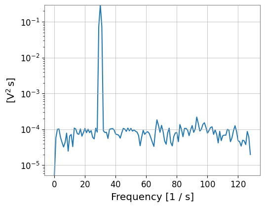
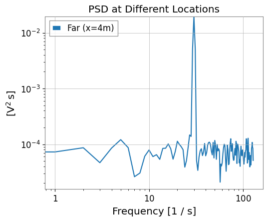
Power Spectral Density (PSD)

Calculate the PSD at a specific location and check frequency components.

# Compare PSD at source position (x=1m) and far field (x=4m)
psd_source = field_sig.psd(point_or_region=(1.0 * u.m, 0.0 * u.m, 0.0 * u.m))
psd_far = field_sig.psd(point_or_region=(4.0 * u.m, 0.0 * u.m, 0.0 * u.m))

plt.figure(figsize=(10, 6))
psd_source.plot(label="Source (x=1m)")
psd_far.plot(label="Far (x=4m)")
plt.xscale("log")
plt.yscale("log")
plt.title("PSD at Different Locations")
plt.legend()
plt.show()

<Figure size 1000x600 with 0 Axes>

Frequency-Space Mapping (Coming Soon)

Note: The plot_freq_space() visualization method is planned for a future release.

For now, you can manually extract and plot frequency-space data using standard matplotlib:

# Extract PSD at different spatial positions
# (Manual visualization example - coming in v0.2.0)

This section will be updated once the visualization API is implemented.

# Visualization method plot_freq_space() will be available in v0.2.0
#
# Example usage (future):
# field_sig.plot_freq_space(
#     space_axis="x",
#     fixed_coords={"y": 0.0 * u.m, "z": 0.0 * u.m},
#     freq_range=(10, 100),
#     log_scale=True,
# )

print("Note: Frequency-space visualization will be added in a future release")

Note: Frequency-space visualization will be added in a future release

Cross-Correlation and Delay Estimation

Calculate cross-correlation between a reference point (source position) and other locations to visualize signal propagation delays.

# plot_cross_correlation() visualization method will be available in v0.2.0
#
# Example usage (future):
# Use x=1.0m (source) as reference point
# ref_point = (1.0 * u.m, 0.0 * u.m, 0.0 * u.m)
#
# # Calculate and plot cross-correlation
# lags, corrs = field_sig.plot_cross_correlation(
#     ref_point=ref_point,
#     scan_axis="x",
#     fixed_coords={"y": 0.0 * u.m, "z": 0.0 * u.m},
#     max_lag=0.5,
# )

print("Note: Cross-correlation visualization will be added in a future release")

Note: Cross-correlation visualization will be added in a future release

The V-shaped pattern shows that the signal propagates from x=1.0m in both directions.

Coherence Map

Display spatial coherence at a specific frequency (here 30Hz).

# plot_coherence_map() visualization method will be available in v0.2.0
#
# Example usage (future):
# field_sig.plot_coherence_map(
#     target_freq=30.0,
#     ref_point=ref_point,
#     scan_axis="x",
#     fixed_coords={"y": 0.0 * u.m, "z": 0.0 * u.m},
# )

print("Note: Coherence map visualization will be added in a future release")

Note: Coherence map visualization will be added in a future release

6. Verification of Numerical Invariants

To verify the accuracy of FFT transformations, we confirm that round-trip transformations can reconstruct the original data.

# Time FFT invariant check: ifft_time(fft_time(f)) ≈ f
np.random.seed(42)
data_test = np.random.randn(64, 4, 4, 4)
field_test = ScalarField(
    data_test,
    unit=u.V,
    axis0=np.arange(64) * 0.01 * u.s,
    axis1=np.arange(4) * u.m,
    axis2=np.arange(4) * u.m,
    axis3=np.arange(4) * u.m,
    axis_names=["t", "x", "y", "z"],
    axis0_domain="time",
    space_domain="real",
)

# Round-trip
field_roundtrip = field_test.fft_time().ifft_time()

# Check
max_error_time = np.max(np.abs(field_test.value - field_roundtrip.value.real))
print(f"Time FFT Round-trip max error: {max_error_time:.2e}")
assert max_error_time < 1e-10, "Time FFT round-trip failed!"
print("Time FFT invariant check: PASSED")

Time FFT Round-trip max error: 9.99e-16
Time FFT invariant check: PASSED