Note

This page was generated from a Jupyter Notebook. Download the notebook (.ipynb)

# Skipped in CI: Colab/bootstrap dependency install cell.

FrequencySeries: Basics

This notebook introduces the new methods and features of the FrequencySeries class extended in gwexpy. We will focus on handling complex spectra, calculus operations, filtering (smoothing), and integration with other libraries.

import warnings

warnings.filterwarnings("ignore", category=UserWarning)
warnings.filterwarnings("ignore", category=DeprecationWarning)

import matplotlib.pyplot as plt
import numpy as np

from gwexpy.frequencyseries import FrequencySeries
from gwexpy.plot import Plot
from gwexpy.timeseries import TimeSeries

plt.rcParams["figure.figsize"] = (10, 6)

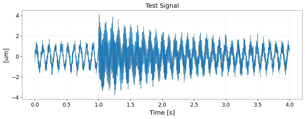
1. Data Preparation

First, we create a FrequencySeries from a TimeSeries using FFT. Here, we generate a test signal with specific frequency components.

fs = 1024
t = np.arange(0, 4, 1 / fs)
exp = np.exp(-t / 1.5)
exp[: int(exp.size / 4)] = 0
data = (
    np.sin(2 * np.pi * 10.1 * t)
    + 5 * exp * np.sin(2 * np.pi * 100.1 * t)
    + np.random.normal(scale=0.3, size=len(t))
)
ts = TimeSeries(data, dt=1 / fs, unit="um", name="Test Signal")
print(ts)

fig, ax = plt.subplots(figsize=(10, 4))
ax.plot(ts.times.value, ts.value, lw=0.8)
ax.set_xlabel("Time [s]")
ax.set_ylabel(f"[{ts.unit}]")
ax.set_title(ts.name)
ax.grid(True, alpha=0.3)
plt.tight_layout()
plt.show()

# Perform FFT to obtain FrequencySeries (using transient mode with padding)
spec = ts.fft(mode="transient", pad_left=1.0, pad_right=1.0, nfft_mode="next_fast_len")
print(f"Type: {type(spec)}")
print(f"Length: {len(spec)}")
print(f"df: {spec.df}")

TimeSeries([ 0.07264356,  0.21497218, -0.50823175, ...,
             0.84230356,  0.74439821,  0.64896141],
           unit: um,
           t0: 0.0 s,
           dt: 0.0009765625 s,
           name: Test Signal,
           channel: None)

Type: <class 'gwexpy.frequencyseries.frequencyseries.FrequencySeries'>
Length: 3073
df: 0.16666666666666666 Hz

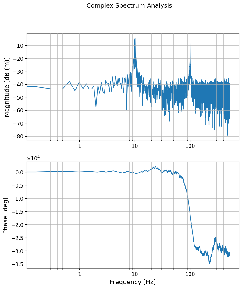
2. Visualization and Conversion of Complex Spectra

Phase and Amplitude

Using the phase(), degree(), and to_db() methods, you can convert complex spectra into intuitive units.

# Convert amplitude to dB (ref=1.0, 20*log10)
spec_db = spec.to_db()

# Get phase (in degrees, unwrap=True for continuity)
spec_phase = spec.degree(unwrap=True)

plot = Plot(spec_db, spec_phase, separate=True, sharex=True, xscale="log")
ax = plot.axes
ax[0].set_ylabel("Magnitude [dB (m)]")
ax[0].grid(True, which="both")

ax[1].set_ylabel("Phase [deg]")
ax[1].set_xlabel("Frequency [Hz]")
ax[1].grid(True, which="both")
plot.figure.suptitle("Complex Spectrum Analysis")
plot.show()

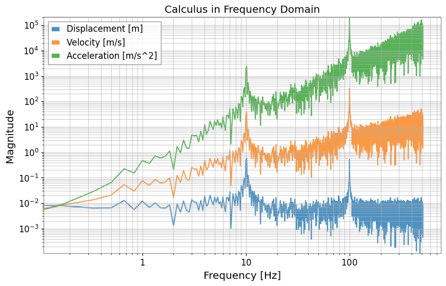
3. Calculus in Frequency Domain

The differentiate() and integrate() methods allow you to perform differentiation and integration in the frequency domain. You can specify the order using the order argument (default is 1). This feature makes it easy to convert between displacement, velocity, and acceleration (multiplication/division by \((2 \pi i f)^n\)).

# Differentiate from displacement (m) to velocity (m/s) (order=1)
vel_spec = spec.differentiate()

# Differentiate from displacement (m) to acceleration (m/s^2) (order=2)
accel_spec = spec.differentiate(order=2)

# Integration is also possible: acceleration -> velocity
vel_from_accel = accel_spec.integrate()

plot = Plot(
    spec.abs(), vel_spec.abs(), accel_spec.abs(), xscale="log", yscale="log", alpha=0.8
)
ax = plot.gca()
ax.get_lines()[0].set_label("Displacement [m]")
ax.get_lines()[1].set_label("Velocity [m/s]")
ax.get_lines()[2].set_label("Acceleration [m/s^2]")
ax.legend()
ax.grid(True, which="both")
ax.set_title("Calculus in Frequency Domain")
ax.set_ylabel("Magnitude")
plot.show()

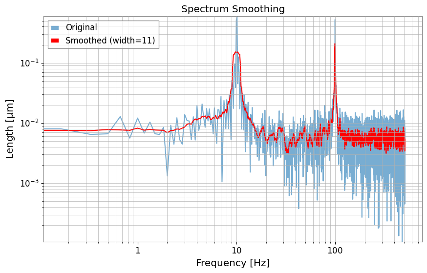
4. Spectrum Smoothing and Peak Detection

Smoothing

The smooth() method enables smoothing of the spectrum using moving averages and other techniques.

# Smooth in amplitude domain with 11 samples
spec_smooth = spec.smooth(width=11)

plot = Plot(spec.abs(), spec_smooth.abs(), xscale="log", yscale="log")
ax = plot.gca()
ax.get_lines()[0].set_label("Original")
ax.get_lines()[0].set_alpha(0.6)
ax.get_lines()[1].set_label("Smoothed (width=11)")
ax.get_lines()[1].set_color("red")
ax.legend()
ax.grid(True, which="both")
ax.set_title("Spectrum Smoothing")
plot.show()

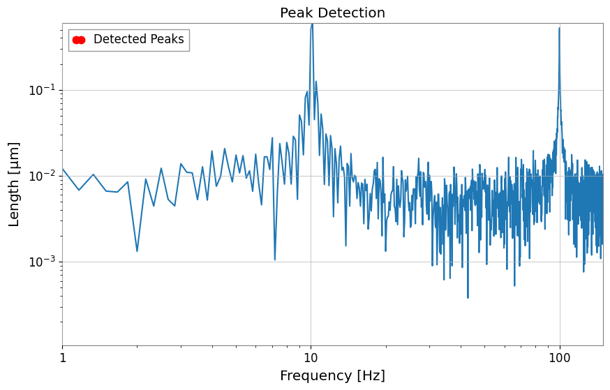
Peak Detection

The find_peaks() method wraps scipy.signal.find_peaks, making it easy to extract peaks above a specific threshold.

# Find peaks with amplitude >= 0.2
peaks, props = spec.find_peaks(threshold=0.2)

plot = Plot(spec.abs())
ax = plot.gca()
ax.plot(
    peaks.abs(), color="red", marker=".", ms=15, lw=0, zorder=3, label="Detected Peaks"
)
ax.set_xlim(1, 150)
ax.set_xscale("log")
ax.set_yscale("log")
ax.set_title("Peak Detection")
ax.legend()
plot.show()

5. Advanced Analysis Features

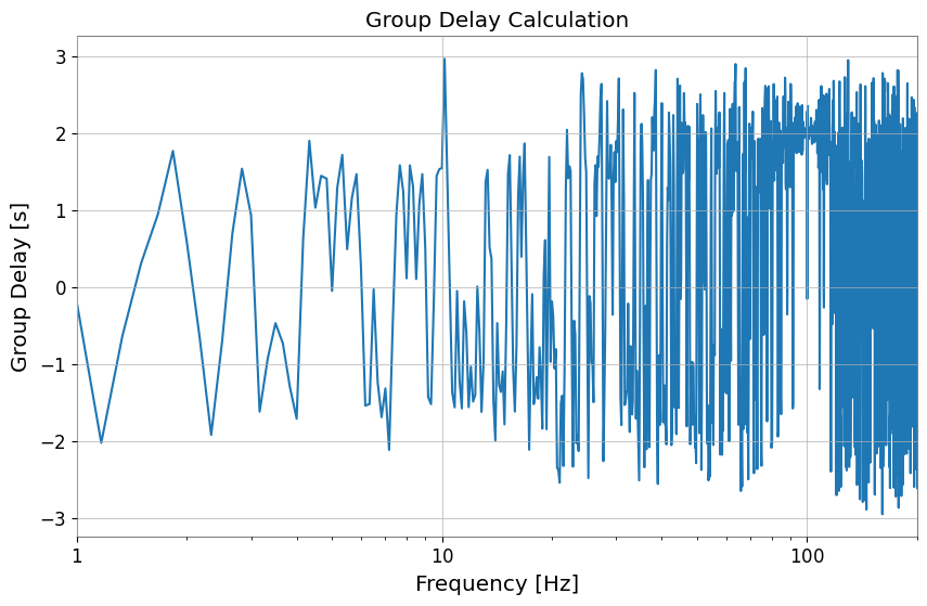
Group Delay

The group_delay() method calculates the group delay (delay of the signal envelope) from the frequency derivative of the phase.

gd = spec.group_delay()

plot = Plot(gd)
ax = plot.gca()
ax.set_ylabel("Group Delay [s]")
ax.set_xlabel("Frequency [Hz]")
ax.set_xlim(1, 200)
ax.set_title("Group Delay Calculation")
plot.show()

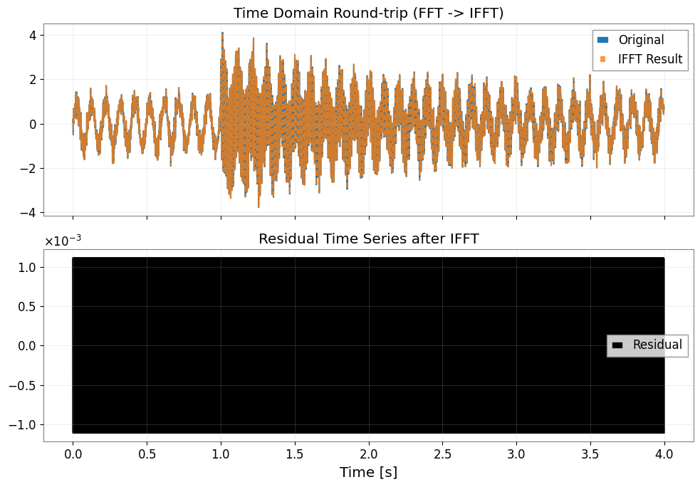
Inverse FFT (ifft)

The ifft() method returns a TimeSeries. Even for results from FFT with mode="transient", it can inherit the information and control restoration to the original length (trim=True).

# Convert back to TimeSeries with inverse FFT
# mode="auto" reads the transient information from the input FrequencySeries and processes it appropriately
inv_ts = spec.ifft(mode="auto")
red_ts = inv_ts - ts

fig, axes = plt.subplots(2, 1, figsize=(10, 7), sharex=True)
axes[0].plot(ts.times.value, ts.value, label="Original")
axes[0].plot(inv_ts.times.value, inv_ts.value, "--", alpha=0.8, label="IFFT Result")
axes[0].set_title("Time Domain Round-trip (FFT -> IFFT)")
axes[0].legend()
axes[0].grid(True, alpha=0.3)

axes[1].plot(red_ts.times.value, red_ts.value, color="black", label="Residual")
axes[1].set_title("Residual Time Series after IFFT")
axes[1].set_xlabel("Time [s]")
axes[1].legend()
axes[1].grid(True, alpha=0.3)

plt.tight_layout()
plt.show()

6. Integration with Other Libraries

Interconversion with Pandas, xarray, and control libraries has been added.

# Convert to Pandas Series
pd_series = spec.to_pandas()
print("Pandas index sample:", pd_series.index[:5])
display(pd_series)

# Convert to xarray DataArray
try:
    da = spec.to_xarray()
    print("xarray coord name:", list(da.coords))
    display(da)
except ImportError:
    print("xarray not installed, skipping DataArray conversion.")

# Convert to control.FRD (can be used for control system analysis)
try:
    from control import FRD

    _ = FRD
    frd_obj = spec.to_control_frd()
    print("Successfully converted to control.FRD")
    display(frd_obj)
except ImportError:
    print("python-control library not installed")

Pandas index sample: Index([0.0, 0.16666666666666666, 0.3333333333333333, 0.5, 0.6666666666666666], dtype='float64', name='frequency')

frequency
0.000000      0.001313+0.000000j
0.166667      0.008022+0.000205j
0.333333     -0.006485-0.000158j
0.500000     -0.003937+0.005328j
0.666667     -0.008695-0.009396j
                     ...
511.333333    0.006786+0.000330j
511.500000    0.002127+0.002070j
511.666667   -0.006518+0.000255j
511.833333    0.005030-0.003855j
512.000000   -0.002221+0.000000j
Name: Test Signal, Length: 3073, dtype: complex128

xarray not installed, skipping DataArray conversion.
Successfully converted to control.FRD

FrequencyResponseData(
array([[[ 0.00131291+0.j        ,  0.00802248+0.0002051j ,
         -0.00648467-0.00015793j, ...,
         -0.00651778+0.00025502j,  0.00502963-0.00385452j,
         -0.00222119+0.j        ]]], shape=(1, 1, 3073)),
array([0.00000000e+00, 1.66666667e-01, 3.33333333e-01, ...,
       5.11666667e+02, 5.11833333e+02, 5.12000000e+02],
      shape=(3073,)),
outputs=1, inputs=1)

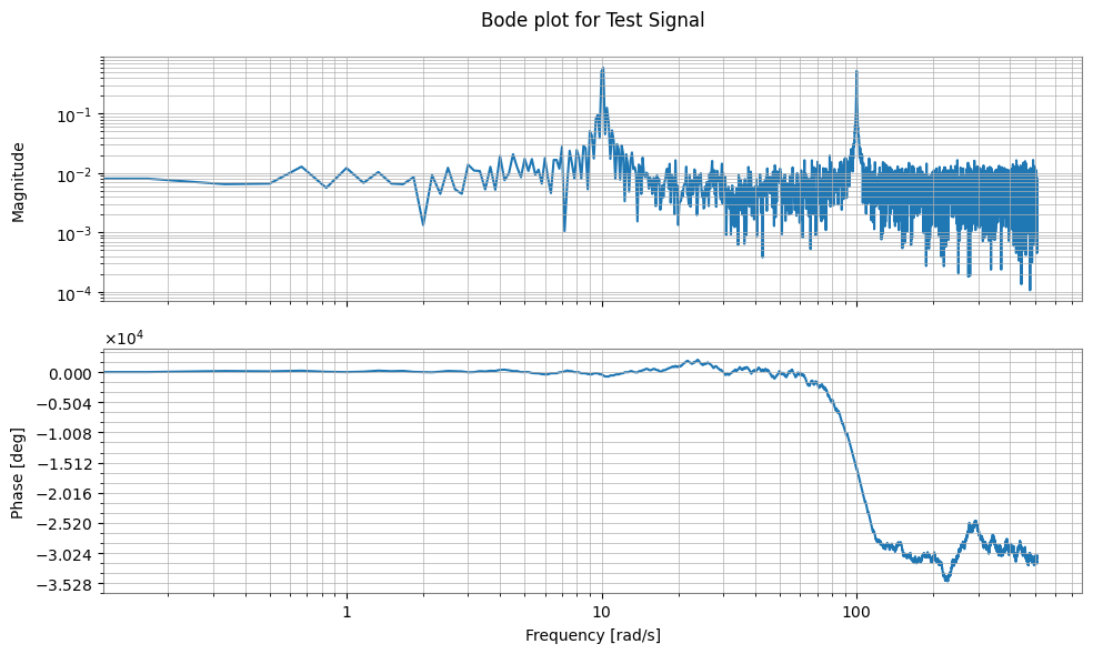
7. Integration with Python Control Library

Interconversion with the Frequency Response Data (FRD) object from the control library, which is standard in the field of control engineering, is possible. This allows transfer functions measured with GWexpy to be directly used for control system design and analysis.

try:
    import control

    # Convert FrequencySeries -> control.FRD
    # Specifying frequency_unit="Hz" appropriately converts to rad/s internally
    frd_sys = spec.to_control_frd(frequency_unit="Hz")

    print("\n--- Converted to Control FRD ---")
    print(str(frd_sys)[:1000] + "\n... (truncated) ...")

    # Plot Bode diagram (control library functionality)
    control.bode(frd_sys)  # (executable if plotting environment is available)

    # Restore control.FRD -> FrequencySeries
    fs_restored = FrequencySeries.from_control_frd(frd_sys, frequency_unit="Hz")

    print("\n--- Restored FrequencySeries ---")
    print(fs_restored)

except ImportError:
    print("Python Control Systems Library is not installed.")

--- Converted to Control FRD ---
<FrequencyResponseData>: sys[1]
Inputs (1): ['u[0]']
Outputs (1): ['y[0]']

Freq [rad/s]  Response
------------  ---------------------
       0.000    0.001313        +0j
       0.167    0.008022+0.0002051j
       0.333   -0.006485-0.0001579j
       0.500   -0.003937 +0.005328j
       0.667   -0.008695 -0.009396j
       0.833    0.003763 +0.004179j
       1.000      0.0121-0.0006805j
       1.167    0.002131 +0.006472j
       1.333   -0.005326 -0.008895j
       1.500   -0.005594 +0.003571j
       1.667   -0.006006 -0.002407j
       1.833    0.007016 +0.004783j
       2.000    0.001301-0.0002375j
       2.167    0.007328 -0.005517j
       2.333    0.001877 +0.004027j
       2.500    -0.01194 -0.002746j
       2.667   -0.004569 +0.002705j
       2.833   -0.001497 +0.004205j
       3.000     0.01129 -0.007956j
       3.167     0.01097 -0.000537j
       3.333    -0.01006 +0.003942j
       3.500   -0.001644  +0.00502j
       3.667    -0.01047 -0.007232j
       3.833   -0.005027 -0.001405j

... (truncated) ...

--- Restored FrequencySeries ---
FrequencySeries([ 0.00131291+0.j        ,
                  0.00802248+0.0002051j ,
                 -0.00648467-0.00015793j, ...,
                 -0.00651778+0.00025502j,
                  0.00502963-0.00385452j,
                 -0.00222119+0.j        ],
                unit: dimensionless,
                f0: 0.0 Hz,
                df: 0.02652582384864922 Hz,
                epoch: None,
                name: None,
                channel: None)

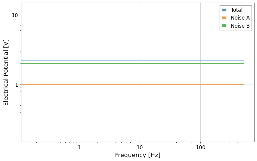
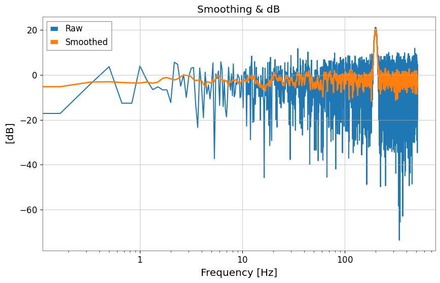
8. Quadrature Sum

This feature calculates the sum of orthogonal components.

# Generate noisy data
np.random.seed(42)
f = spec.frequencies.value
noise = np.abs(np.random.randn(f.size))
peak = 10.0 * np.exp(-((f - 200) ** 2) / 50.0)
data = noise + peak

raw = FrequencySeries(data, frequencies=f, unit="V", name="Raw Data")

# Smooth
smoothed = raw.smooth(width=10, method="amplitude")
smoothed.name = "Smoothed"

# Convert to dB
raw_db = raw.to_db()
smoothed_db = smoothed.to_db()
raw_db.name = "Raw (dB)"
smoothed_db.name = "Smoothed (dB)"

plot = raw_db.plot(label="Raw", title="Smoothing & dB")
ax = plot.gca()
ax.plot(smoothed_db, label="Smoothed", linewidth=2)
ax.legend()
plot.show()
plt.close()

# Quadrature Sum (Noise Budget example)
noise_a = FrequencySeries(np.ones_like(f), frequencies=f, unit="V", name="Noise A")
noise_b = FrequencySeries(np.ones_like(f) * 2, frequencies=f, unit="V", name="Noise B")

total = noise_a.quadrature_sum(noise_b)
print(f"Noise A: {noise_a.value[0]}, Noise B: {noise_b.value[0]}")
print(f"Total (Sqrt Sum): {total.value[0]}")
Plot(total, noise_a, noise_b, alpha=0.8)
plt.legend(["Total", "Noise A", "Noise B"])
plt.xscale("log")
plt.yscale("log")
plt.show()

Noise A: 1.0, Noise B: 2.0
Total (Sqrt Sum): 2.23606797749979