Note

This page was generated from a Jupyter Notebook. Download the notebook (.ipynb)

# Skipped in CI: Colab/bootstrap dependency install cell.

TimeSeries: Basics

This notebook introduces the new methods added to the TimeSeries class in gwexpy, an extension of gwpy, and explains how to use them.

gwexpy maintains high compatibility with GWpy while significantly enhancing signal processing, statistical analysis, and interoperability with other libraries.

Table of Contents

1. Environment Setup

2. Signal Processing and Demodulation (Hilbert, Phase, Demodulation)

3. Spectral Analysis and Correlation (FFT, Transfer Function, xcorr)

4. Hilbert-Huang Transform (HHT)

5. Statistics and Preprocessing (Impute, Standardize, ARIMA, Hurst, Rolling)

6. Resampling and Reindexing (asfreq, resample)

7. Function Fitting (fit)

8. Interoperability (Pandas, Xarray, Torch, and more)

1. Environment Setup

First, we import the necessary libraries and generate sample data for demonstration.

import warnings

warnings.filterwarnings("ignore", category=UserWarning)
warnings.filterwarnings("ignore", category=DeprecationWarning)

import matplotlib.pyplot as plt
import numpy as np
from astropy import units as u

from gwexpy.noise.wave import chirp, exponential, gaussian, sine
from gwexpy.plot import Plot
from gwexpy.timeseries import TimeSeries

# Generate two toy channels: one nearly stationary line and one drifting chirp so later diagnostics have a clear physical target.
fs = 100
duration = 5.0
# Restore 't' for compatibility with downstream cells if they use it
t = np.arange(0, duration, 1 / fs)

# Sensor 1 behaves like a stable calibration line plus measurement noise, which is useful as a demodulation reference.
s1 = sine(duration=duration, sample_rate=fs, frequency=10, amplitude=1.0)
n1 = gaussian(duration=duration, sample_rate=fs, std=0.2)
ts1 = s1 + n1
ts1.name = "Sensor 1"
ts1.override_unit("V")

# Sensor 2 mimics a non-stationary line whose frequency sweeps and whose amplitude grows, so Hilbert-based tracking has a meaningful physical trend to recover.
s2 = chirp(duration=duration, sample_rate=fs, f0=5, f1=25, t1=duration)
env = exponential(
    duration=duration, sample_rate=fs, tau=2.0, decay=False, amplitude=0.2
)
ts2 = s2 * env
ts2.name = "Chirp Signal"
ts2.override_unit("V")

2. Signal Processing and Demodulation

gwexpy integrates Hilbert transforms, envelope calculations, instantaneous frequency computation, and demodulation functions like lock-in amplifiers.

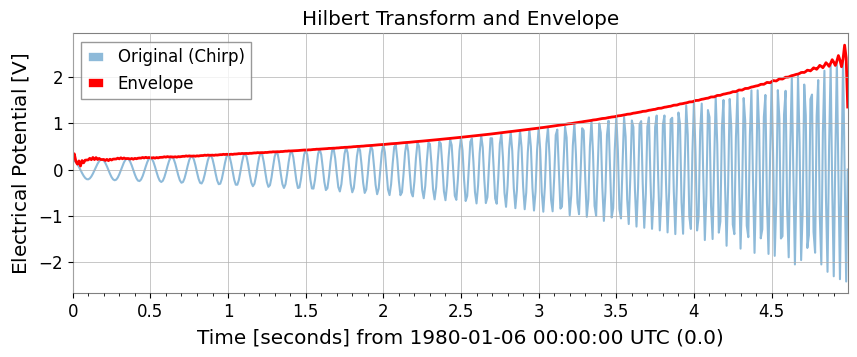
Hilbert Transform and Envelope

Use hilbert and envelope.

# Build the analytic signal so amplitude and phase can be separated without cancelling positive and negative frequency content.
ts_analytic = ts2.hilbert()
# The envelope isolates the slow amplitude modulation riding on top of the oscillatory carrier.
ts_env = ts2.envelope()

plot = Plot(ts2, ts_env, figsize=(10, 4))
ax = plot.gca()
ax.get_lines()[0].set_label("Original (Chirp)")
ax.get_lines()[0].set_alpha(0.5)
ax.get_lines()[1].set_label("Envelope")
ax.get_lines()[1].set_color("red")
ax.get_lines()[1].set_linewidth(2)
ax.legend()
ax.set_title("Hilbert Transform and Envelope")
plt.show()

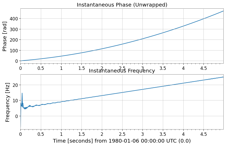
Instantaneous Phase and Instantaneous Frequency

Use instantaneous_phase and instantaneous_frequency. You can specify phase unwrapping (unwrap) and degree units (deg).

# Unwrap the phase so the chirp appears as continuous phase accumulation instead of artificial 2pi jumps.
phase_rad = ts2.instantaneous_phase(unwrap=True)
phase_deg = ts2.instantaneous_phase(deg=True, unwrap=True)

# Convert the phase slope into instantaneous frequency to follow the drifting line in time.
freq = ts2.instantaneous_frequency()

plot = Plot(phase_rad, freq, separate=True, sharex=True, figsize=(10, 6))
ax = plot.axes
ax[0].set_ylabel("Phase [rad]")
ax[0].set_title("Instantaneous Phase (Unwrapped)")
ax[1].set_ylabel("Frequency [Hz]")
ax[1].set_title("Instantaneous Frequency")
plt.show()

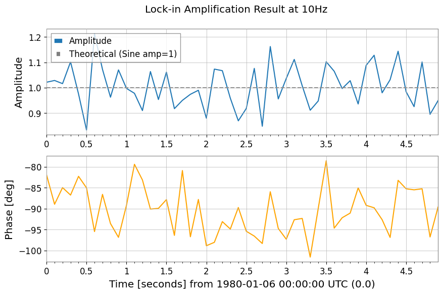
Mixing and Demodulation (Mix-down, Baseband, Lock-in)

Functions for extracting specific frequency components or bringing them down to baseband.

# 1. Mix down to 10 Hz so the narrowband line is shifted to baseband, where slow amplitude and phase changes are easier to measure.
ts_mixed = ts1.mix_down(f0=10)

# 2. Baseband adds low-pass filtering and decimation so the retained samples describe only the slow envelope, not the carrier itself.
ts_base = ts1.baseband(f0=10, lowpass=5, output_rate=20)

# 3. Lock-in detection averages against a phase-matched reference, which suppresses broadband noise while preserving the coherent 10 Hz component.
amp, ph = ts1.lock_in(f0=10, stride=0.1)  # Output average every 0.1 seconds
res_complex = ts1.lock_in(
    f0=10, stride=0.1, output="complex"
)  # Output as complex numbers

print(amp)

plot = Plot(amp, ph, separate=True, sharex=True, figsize=(10, 6))
ax = plot.axes
ax[0].get_lines()[0].set_label("Amplitude")
ax[0].axhline(1.0, color="gray", linestyle="--", label="Theoretical (Sine amp=1)")
ax[0].set_ylabel("Amplitude")
ax[0].legend()
ax[1].get_lines()[0].set_color("orange")
ax[1].get_lines()[0].set_label("Phase [deg]")
ax[1].set_ylabel("Phase [deg]")
plot.figure.suptitle("Lock-in Amplification Result at 10Hz")
plt.show()

TimeSeries([1.02125098, 1.02816908, 1.01569884, 1.10170511,
            0.9748796 , 0.83238678, 1.21296852, 1.07186959,
            0.96209319, 1.06991493, 0.99690912, 0.97742513,
            0.90919853, 1.06345248, 0.95293007, 1.06111695,
            0.91684155, 0.9495788 , 0.97350793, 0.98943324,
            0.87912426, 1.07313197, 1.06691906, 0.95801234,
            0.86871153, 0.91762836, 1.07592713, 0.84729463,
            1.16227649, 0.95528444, 1.03600341, 1.11143565,
            1.00699916, 0.91062728, 0.94706259, 1.10218972,
            1.06468818, 0.99637142, 1.02737997, 0.93524989,
            1.08785347, 1.12791979, 0.97941365, 1.03120584,
            1.14380495, 0.9838363 , 0.92467013, 1.10117498,
            0.89458811, 0.94843371],
           unit: V,
           t0: 0.0 s,
           dt: 0.1 s,
           name: Sensor 1,
           channel: None)

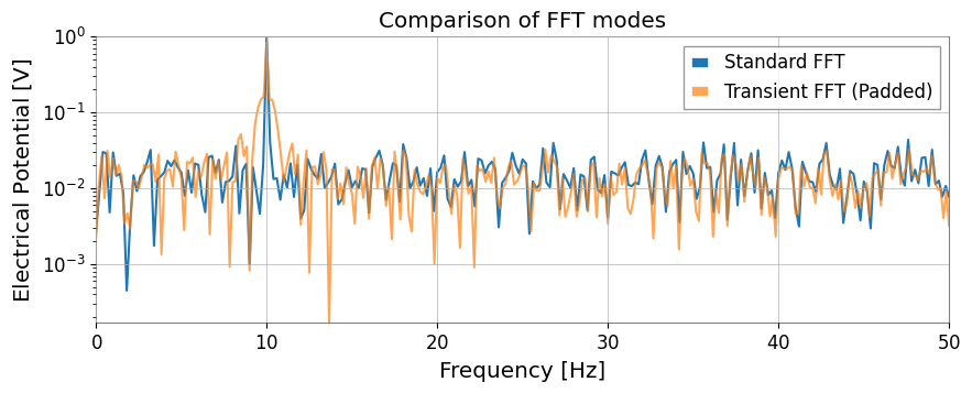
3. Spectral Analysis and CorrelationWhile inheriting GWpy’s functionality, mode="transient" FFT for transient signals and transfer function calculation via direct FFT ratio have been added.

Extended FFTUsing mode="transient" enables zero-padding, adjustment to fast lengths, and individual left/right padding specifications.

# Standard FFT is appropriate when the signal is roughly stationary over the full record and you want GWpy-compatible normalization.
fs_gwpy = ts1.fft()

# Transient mode is better for short-lived responses because padding reduces edge leakage that would otherwise distort amplitudes.
# pad_left/pad_right extend the event in time, and nfft_mode="next_fast_len" keeps that protection computationally cheap.
fs_trans = ts1.fft(
    mode="transient", pad_left=0.5, pad_right=0.5, nfft_mode="next_fast_len"
)

plot = Plot(fs_gwpy.abs(), fs_trans.abs(), yscale="log", xlim=(0, 50), figsize=(10, 4))
ax = plot.gca()
ax.get_lines()[0].set_label("Standard FFT")
ax.get_lines()[1].set_label("Transient FFT (Padded)")
ax.get_lines()[1].set_alpha(0.7)
ax.legend()
ax.set_title("Comparison of FFT modes")
plt.show()

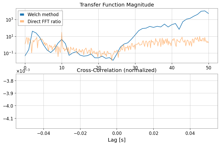
Transfer Function and Cross-Correlation (xcorr)With transfer_function, you can choose not only the Welch method (mode="steady") but also direct FFT ratio (mode="transient").

# Estimate the transfer function to ask whether Sensor 1 can linearly explain features in the chirping channel across frequency.
tf_welch = ts2.transfer_function(ts1, fftlength=1)
tf_fft = ts2.transfer_function(
    ts1, mode="transient"
)  # Full-span FFT ratio (useful for transient response analysis)

# Cross-correlation checks whether the two channels line up in time, which is a first sanity check before treating one as a witness for the other.
corr = ts1.xcorr(ts2, maxlag=0.5, normalize="coeff")

plot = Plot(figsize=(10, 6))
ax1 = plot.add_subplot(2, 1, 1)
ax1.semilogy(tf_welch.frequencies, np.abs(tf_welch), label="Welch method")
ax1.semilogy(tf_fft.frequencies, np.abs(tf_fft), label="Direct FFT ratio", alpha=0.5)
ax1.set_title("Transfer Function Magnitude")
ax1.legend()

ax2 = plot.add_subplot(2, 1, 2)
lag = corr.times.value - corr.t0.value
ax2.plot(lag, corr)
ax2.set_title("Cross-Correlation (normalized)")
ax2.set_xlabel("Lag [s]")
plt.show()

STLT (Short-Time Laplace Transform)STLT (Short-Time Laplace Transform) is a transform for extracting local structures that change over time in a signal.In gwexpy, the STLT result is a 3D transform with axes (time × sigma × frequency), represented by TimePlaneTransform / LaplaceGram.Below is an example of calculating STLT using the stlt method and extracting a slice (Plane2D) at a specific time.This example also demonstrates specifying frequencies (Hz) to evaluate STLT at arbitrary frequency points.

# Data preparation (for demonstration)
import numpy as np

from gwexpy.plot import Plot

t = np.linspace(0, 10, 1000)
data = TimeSeries(np.sin(2 * np.pi * 1 * t), times=t * u.s, unit="V", name="Demo Data")

# STLT
# stride: time step, window: analysis window length
freqs = np.array([0.5, 1.0, 1.5])  # Hz
stlt_result = data.stlt(stride="0.5s", window="2s", frequencies=freqs)

print(f"Kind: {stlt_result.kind}")
print(f"Shape: {stlt_result.shape} (Time x Sigma x Frequency)")
print(f"Time Axis: {len(stlt_result.times)} steps")
print(f"Sigma Axis: {len(stlt_result.axis1.index)} bins")
print(f"Frequency Axis: {len(stlt_result.axis2.index)} bins")

# Extract plane at specific time (t=5.0s)
plane_at_5s = stlt_result.at_time(5.0 * u.s)
print(f"Plane at 5.0s shape: {plane_at_5s.shape}")

# Plane2D Confirm behavior as Plane2D
print(f"Axis 1: {plane_at_5s.axis1.name}")
print(f"Axis 2: {plane_at_5s.axis2.name}")

Kind: stlt
Shape: (17, 1, 3) (Time x Sigma x Frequency)
Time Axis: 17 steps
Sigma Axis: 1 bins
Frequency Axis: 3 bins
Plane at 5.0s shape: (1, 3)
Axis 1: sigma
Axis 2: frequency

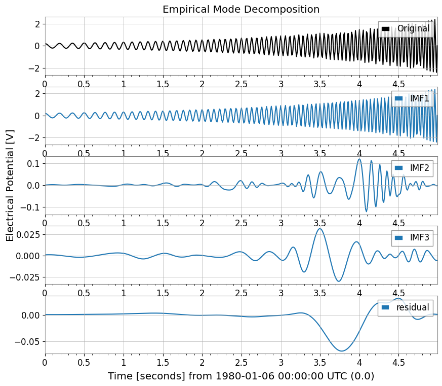
4. Hilbert-Huang Transform (HHT)Hilbert-Huang Transform (HHT) functionality for nonlinear and non-stationary signal analysis.Combines Empirical Mode Decomposition (EMD) and Hilbert spectral analysis.

import warnings

with warnings.catch_warnings():
    warnings.simplefilter('ignore')

    # HHT (Hilbert-Huang Transform)
    # Execute Empirical Mode Decomposition (EMD) and extract IMFs (Intrinsic Mode Functions)
    # Note: Requires PyEMD (EMD-signal) : `pip install EMD-signal`

    try:
        import os

        os.environ["TF_CPP_MIN_LOG_LEVEL"] = "2"
        # EMDExecute EMD (returns dictionary)
        # method="emd" (standard EMD) or "eemd" (Ensemble EMD)
        # Here we use ts2 (example with chirp signal)
        imfs = ts2.emd(method="emd", max_imf=3)

        print(f"Extracted IMFs: {list(imfs.keys())}")

        # Plot IMFs
        sorted_keys = sorted(
        [k for k in imfs.keys() if k.startswith("IMF")], key=lambda x: int(x[3:])
        )
        if "residual" in imfs:
            sorted_keys.append("residual")

        # gwexpy.plot.Plot for batch plotting
        plot_data = [ts2] + [imfs[k] for k in sorted_keys]
        plot = Plot(*plot_data, separate=True, sharex=True, figsize=(10, 8))

        # Original settings
        ax0 = plot.axes[0]
        ax0.get_lines()[0].set_label("Original")
        ax0.get_lines()[0].set_color("black")
        ax0.legend(loc="upper right")
        ax0.set_title("Empirical Mode Decomposition")

        # IMF settings
        for i, key in enumerate(sorted_keys):
            ax = plot.axes[i + 1]
            ax.get_lines()[0].set_label(key)
            ax.legend(loc="upper right")

        plt.show()

    except ImportError:
        print("EMD-signal not installed. Skipping HHT demo.")
    except Exception as e:
        print(f"HHT Error: {e}")

Extracted IMFs: ['IMF1', 'IMF2', 'IMF3', 'residual']

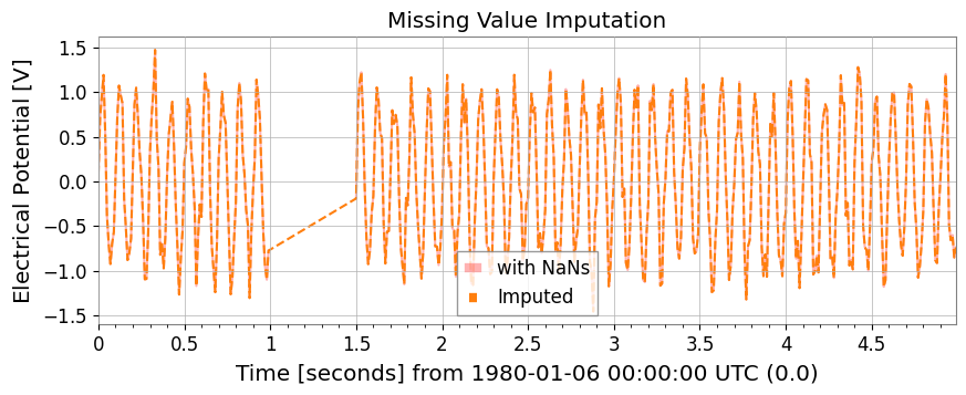
5. Statistics and PreprocessingMissing value imputation, standardization, ARIMA models, Hurst exponent, and rolling statistics are available as TimeSeries methods.

# Test data with missing values
ts_nan = ts1.copy()
ts_nan.value[100:150] = np.nan

# 1. impute: Missing value imputation (interpolation, etc.)
ts_imputed = ts_nan.impute(method="interpolate")

# 2. standardize: Standardization (z-score, robust, etc.)
ts_z = ts1.standardize(method="zscore")
ts_robust = ts1.standardize(method="zscore", robust=True)  # Use Median/IQR

plot = Plot(ts_nan, ts_imputed, figsize=(10, 4))
ax = plot.gca()
ax.get_lines()[0].set_label("with NaNs")
ax.get_lines()[0].set_color("red")
ax.get_lines()[0].set_alpha(0.3)
ax.get_lines()[1].set_label("Imputed")
ax.get_lines()[1].set_linestyle("--")
ax.legend()
ax.set_title("Missing Value Imputation")
plt.show()

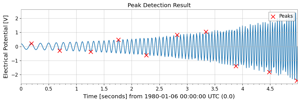
Peak Detection (Find Peaks)Wraps scipy.signal.find_peaks to detect peaks in time series data.

# Peak Detection (Find Peaks)
# height, threshold, distance, prominence, width such asCan specify parameters such as
# Can also specify thresholds with units

# ts2 (Chirp + Sine) Find peaks in
peaks, props = ts2.find_peaks(height=0.0, distance=50)

print(f"Found {len(peaks)} peaks")
if len(peaks) > 0:
    print("First 5 peaks:", peaks[:5])

# Plot
plot = ts2.plot(figsize=(12, 4))
ax = plot.gca()
ax.scatter(
    peaks.times.value,
    peaks.value,
    marker="x",
    color="red",
    s=100,
    label="Peaks",
    zorder=10,
)
ax.legend(loc="upper right")
ax.set_title("Peak Detection Result")
plt.show()

Found 10 peaks
First 5 peaks: TimeSeries([ 0.21779568, -0.28157556, -0.37097234,  0.48196067,
            -0.61630987],
           unit: V,
           t0: 0.19 s,
           dt: 0.51 s,
           name: Chirp Signal_peaks,
           channel: None)

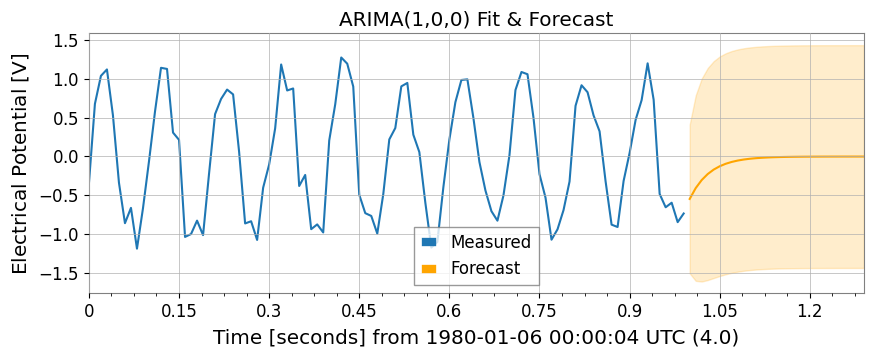
ARIMA Model and Hurst ExponentNote: These features require libraries such as statsmodels and hurst.

import warnings

with warnings.catch_warnings():
    warnings.simplefilter('ignore')

    try:
        import os

        os.environ["TF_CPP_MIN_LOG_LEVEL"] = "2"
        # 3. fit_arima: ARIMA(1,0,0) fitting and forecasting
        model = ts1.fit_arima(order=(1, 0, 0))
        resid = model.residuals()
        forecast, conf = model.forecast(steps=30)

        plot = Plot(ts1.tail(100), forecast, figsize=(10, 4))
        ax = plot.gca()
        ax.get_lines()[0].set_label("Measured")
        ax.get_lines()[1].set_label("Forecast")
        ax.get_lines()[1].set_color("orange")

        # Fill between
        ax.fill_between(
        conf["lower"].times.value,
        conf["lower"].value,
        conf["upper"].value,
        alpha=0.2,
        color="orange",
        )

        ax.set_title("ARIMA(1,0,0) Fit & Forecast")
        ax.legend()
        plt.show()
    except Exception as e:
        print(f"ARIMA skipping: {e}")

    try:
        import os

        os.environ["TF_CPP_MIN_LOG_LEVEL"] = "2"
        # 4. hurst / local_hurst: Hurst exponent (indicator of long-range correlation)
        h_val = ts1.hurst()
        h_detail = ts1.hurst(return_details=True)  # With detailed information
        h_local = ts1.local_hurst(window=1.0)  # Evolution with 1-second window

        plot = Plot(h_local, figsize=(10, 4))
        ax = plot.gca()
        ax.get_lines()[0].set_label("Local Hurst")
        ax.axhline(h_val, color="red", linestyle="--", label=f"Global H={h_val:.2f}")
        ax.set_ylim(0, 0.2)
        ax.set_title("Hurst Exponent Analysis")
        ax.legend()
        plt.show()
    except Exception as e:
        print(f"Hurst skipping: {e}")

Hurst skipping: No Hurst backend found. Install hurst, hurst-exponent, or exp-hurst.

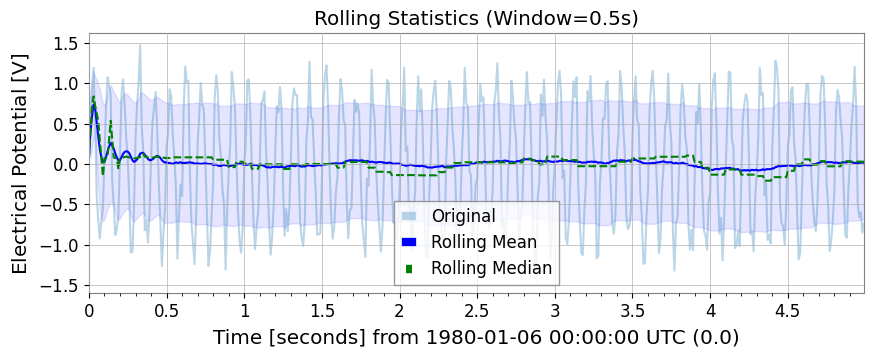
Rolling StatisticsSimilar to Pandas, rolling_mean, std, median, min, max are available.

rw = 0.5 * u.s  # 0.5 second window
rmean = ts1.rolling_mean(rw)
rstd = ts1.rolling_std(rw)
rmed = ts1.rolling_median(rw)
rmin = ts1.rolling_min(rw)
rmax = ts1.rolling_max(rw)

plot = Plot(ts1, rmean, rmed, figsize=(10, 4))
ax = plot.gca()
ax.get_lines()[0].set_label("Original")
ax.get_lines()[0].set_alpha(0.3)
ax.get_lines()[1].set_label("Rolling Mean")
ax.get_lines()[1].set_color("blue")
ax.get_lines()[2].set_label("Rolling Median")
ax.get_lines()[2].set_color("green")
ax.get_lines()[2].set_linestyle("--")
ax.fill_between(
    rmean.times.value,
    rmean.value - rstd.value,
    rmean.value + rstd.value,
    alpha=0.1,
    color="blue",
)
ax.legend()
ax.set_title("Rolling Statistics (Window=0.5s)")
plt.show()

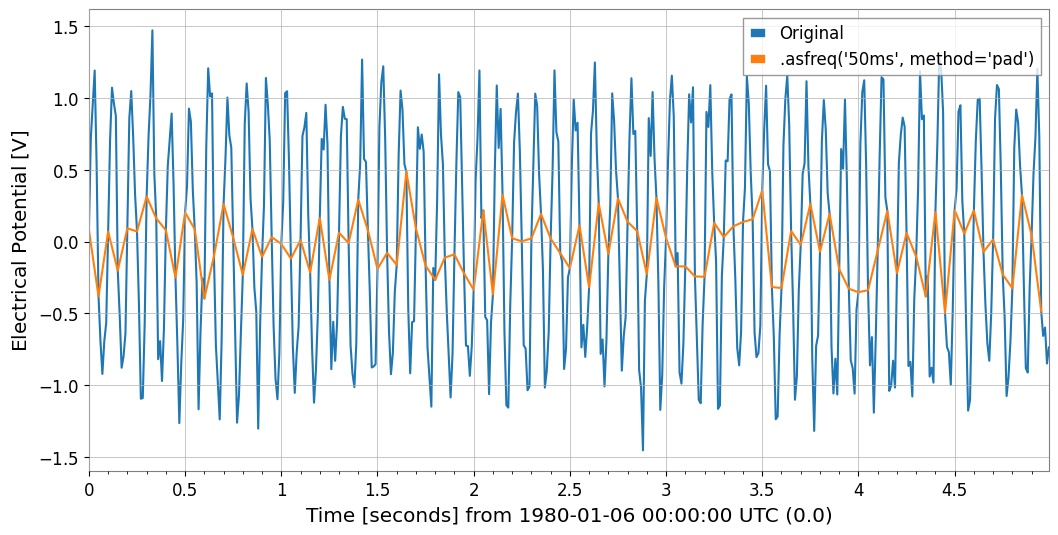
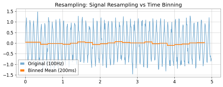
6. Resampling and ReindexingThe asfreq method allows assignment to a fixed grid, and the resample method enables “time bin aggregation”.

# 1. asfreq: Reindex with Pandas-like naming conventions ('50ms' など)
ts_reindexed = ts1.asfreq("50ms", method="pad")
Plot(ts1, ts_reindexed)
plt.legend(["Original", ".asfreq('50ms', method='pad')"])

<matplotlib.legend.Legend at 0x7f1b5156f610>

# 2. resample:
# If you specify a number (10Hz) , signal processing resampling (GWpy standard)
ts_sig = ts1.resample(10)
# If you specify a string ('200ms') , statistics for each time bin (new feature)
ts_binned = ts1.resample("200ms")  # Default is mean

# Plot doesn't have a direct 'step' method equivalent in args, so we use ax.step or pass to plot
# However, kwarg 'drawstyle'='steps-post' works in plot()? gwpy Plot wraps matplotlib.
# Let's assume we can modify axes after creation or use standard plot for simplicity if appropriate, but step is specific.
# Better strategy: Create Plot instance, then use ax.step
plot = Plot(figsize=(10, 4))
ax = plot.gca()
ax.plot(ts1, alpha=0.6, label="Original (100Hz)")
ax.step(
    ts_binned.times,
    ts_binned.value,
    where="post",
    label="Binned Mean (200ms)",
    linewidth=2,
)
ax.legend()
ax.set_title("Resampling: Signal Resampling vs Time Binning")
plt.show()

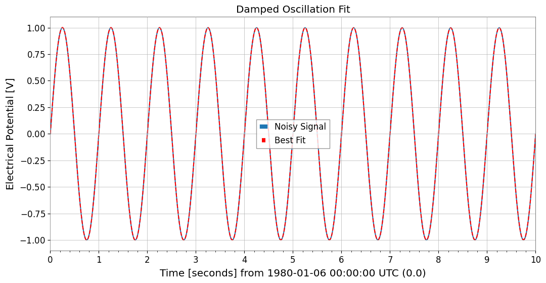
7. Function Fittinggwexpy provides powerful fitting functionality based on iminuit. To avoid polluting GWpy’s original classes, the .fit() method is opt-in.

from gwexpy.fitting.models import damped_oscillation

# Fit with damped oscillation model (pass function directly)
# Initial values: A=0.5, tau=0.5, f=15, phi=0
result = data.fit(damped_oscillation, A=0.5, tau=0.5, f=15, phi=0)

# Display result (iminuit format)
print(result)

# Get best-fit curve
# Note: x_data is the time array corresponding to data points
x_data = data.times.value
best_fit = result.model(x_data)

# Plot
plot = data.plot(label="Noisy Signal")
ax = plot.gca()
ax.plot(data.times, best_fit, label="Best Fit", color="red", linestyle="--")
ax.legend()
ax.set_title("Damped Oscillation Fit")
plt.show()

┌─────────────────────────────────────────────────────────────────────────┐
│                                Migrad                                   │
├──────────────────────────────────┬──────────────────────────────────────┤
│ FCN = 0.0005703 (χ²/ndof = 0.0)  │              Nfcn = 324              │
│ EDM = 0.000176 (Goal: 0.0002)    │                                      │
├──────────────────────────────────┼──────────────────────────────────────┤
│          Valid Minimum           │   Below EDM threshold (goal x 10)    │
├──────────────────────────────────┼──────────────────────────────────────┤
│      No parameters at limit      │           Below call limit           │
├──────────────────────────────────┼──────────────────────────────────────┤
│             Hesse ok             │         Covariance accurate          │
└──────────────────────────────────┴──────────────────────────────────────┘
┌───┬──────┬───────────┬───────────┬────────────┬────────────┬─────────┬─────────┬───────┐
│   │ Name │   Value   │ Hesse Err │ Minos Err- │ Minos Err+ │ Limit-  │ Limit+  │ Fixed │
├───┼──────┼───────────┼───────────┼────────────┼────────────┼─────────┼─────────┼───────┤
│ 0 │ A    │   1.00    │   0.06    │            │            │         │         │       │
│ 1 │ tau  │     0     │  0.06e6   │            │            │         │         │       │
│ 2 │ f    │  1.0000   │  0.0025   │            │            │         │         │       │
│ 3 │ phi  │   -0.00   │   0.09    │            │            │         │         │       │
└───┴──────┴───────────┴───────────┴────────────┴────────────┴─────────┴─────────┴───────┘
┌─────┬─────────────────────────────────────────────────────┐
│     │            A          tau            f          phi │
├─────┼─────────────────────────────────────────────────────┤
│   A │      0.00354 -2.4033829e3         3e-6      -0.0001 │
│ tau │ -2.4033829e3     3.78e+09    -8.714e-3       38.287 │
│   f │         3e-6    -8.714e-3     6.05e-06      -190e-6 │
│ phi │      -0.0001       38.287      -190e-6      0.00796 │
└─────┴─────────────────────────────────────────────────────┘

8. InteroperabilityInterconversion with major data science and machine learning libraries is very smooth.

import warnings

with warnings.catch_warnings():
    warnings.simplefilter('ignore')

    # Pandas & Xarray
    try:
        import os

        os.environ["TF_CPP_MIN_LOG_LEVEL"] = "2"
        df = ts1.to_pandas(index="datetime")
        ts_p = TimeSeries.from_pandas(df)
        print("Pandas interop OK")
        display(df)
    except ImportError:
        pass

    try:
        import os

        os.environ["TF_CPP_MIN_LOG_LEVEL"] = "2"
        xr = ts1.to_xarray()
        ts_xr = TimeSeries.from_xarray(xr)
        print("Xarray interop OK")
        print(xr)
    except ImportError:
        pass

Pandas interop OK

time_utc
1980-01-06 00:00:19+00:00           0.081608
1980-01-06 00:00:19.010000+00:00    0.722866
1980-01-06 00:00:19.020000+00:00    0.953315
1980-01-06 00:00:19.030000+00:00    1.192592
1980-01-06 00:00:19.040000+00:00    0.536523
                                      ...
1980-01-06 00:00:23.950000+00:00   -0.484829
1980-01-06 00:00:23.960000+00:00   -0.656789
1980-01-06 00:00:23.970000+00:00   -0.598129
1980-01-06 00:00:23.980000+00:00   -0.849085
1980-01-06 00:00:23.990000+00:00   -0.737268
Name: Sensor 1, Length: 500, dtype: float64

# SQLite (serialized storage)
import sqlite3

with sqlite3.connect(":memory:") as conn:
    ts1.to_sqlite(conn, series_id="my_sensor")
    ts_sql = TimeSeries.from_sqlite(conn, series_id="my_sensor")
    print(f"SQLite interop OK: {ts_sql.name}")
    display(conn)

SQLite interop OK: my_sensor

<sqlite3.Connection at 0x7f1b50f684f0>

import warnings

with warnings.catch_warnings():
    warnings.simplefilter('ignore')

    # Deep Learning (Torch)
    try:
        import os

        os.environ["TF_CPP_MIN_LOG_LEVEL"] = "2"
        import torch

        _ = torch
        t_torch = ts1.to_torch()
        ts_f_torch = TimeSeries.from_torch(t_torch, t0=ts1.t0, dt=ts1.dt)
        print(f"Torch interop OK (Shape: {t_torch.shape})")
        display(t_torch)
    except ImportError:
        pass

import warnings

with warnings.catch_warnings():
    warnings.simplefilter('ignore')

    # Deep Learning (TensorFlow)
    try:
        import os

        os.environ.setdefault("TF_CPP_MIN_LOG_LEVEL", "3")
        warnings.filterwarnings(
            "ignore", category=UserWarning, module=r"google\.protobuf\..*"
        )
        warnings.filterwarnings(
            "ignore", category=UserWarning, message=r"Protobuf gencode version.*"
        )
        import tensorflow as tf

        _ = tf
        t_tf = ts1.to_tensorflow()
        ts_f_tf = TimeSeries.from_tensorflow(t_tf, t0=ts1.t0, dt=ts1.dt)
        print("TensorFlow interop OK")
        display(t_tf)
    except ImportError:
        pass

import warnings

with warnings.catch_warnings():
    warnings.simplefilter('ignore')

    # ObsPy (seismic waveform and time series analysis)
    try:
        import os

        os.environ["TF_CPP_MIN_LOG_LEVEL"] = "2"
        import obspy

        _ = obspy
        tr = ts1.to_obspy()
        ts_f_obspy = TimeSeries.from_obspy(tr)
        print(f"ObsPy interop OK: {tr.id}")
        display(tr)
    except ImportError:
        pass

Summary

In this tutorial, we have covered the key enhancements in gwexpy.TimeSeries:

• Signal Processing: Hilbert transform, demodulation, and extended FFT modes.

• Statistics: Advanced correlation methods (MIC, Distance Correlation) and ARIMA modeling.

• Data Cleaning: Missing value imputation and standardization.

• Interoperability: Seamless conversion to/from Pandas, Xarray, PyTorch, TensorFlow, and ObsPy.

Next Steps

• Multichannel Data: Learn about TimeSeriesMatrix for handling many channels simultaneously.

• Spectral Analysis: Explore FrequencySeries.

• 4D Fields: Check out ScalarField for spacetime analysis.