Development documentation · 0.2.7 12b76261 · Intro examples tested with 0.2.4 · Version details · Known limitations

Fitting: Basics

Goal: Learn how to fit models to GW data using Ordinary Least Squares (OLS) and Generalized Least Squares (GLS).

GWexpy uses iminuit as its primary optimization engine and provides specialized cost functions for spectral data with correlations.

Install it with the fitting extra before running this notebook: pip install "gwexpy[fitting]".

1. Simple OLS Fit

We start with a simple power-law fit using diagonal errors (OLS).

import warnings


import matplotlib.pyplot as plt
import numpy as np
np.random.seed(42)

from gwexpy.fitting import fit_series

# Generate synthetic data following a power law: y = A * f**alpha
freqs = np.linspace(10, 100, 50)
model = lambda f, A, alpha: A * f**alpha
y_true = model(freqs, 1000.0, -1.5)
y_obs = y_true + np.random.normal(0, 0.3, size=len(freqs))

from gwexpy.frequencyseries import FrequencySeries

psd = FrequencySeries(y_obs, frequencies=freqs)

res = fit_series(psd, model, p0={"A": 100.0, "alpha": -1.0})

res.plot()
plt.xscale("log")
plt.yscale("log")
plt.show()
print(f"Fitted A={res.params['A']:.2f}, alpha={res.params['alpha']:.2f}")

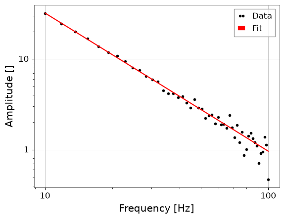
Fitted A=1063.49, alpha=-1.52

2. Generalized Least Squares (GLS)

When data points are correlated (e.g., in a PSD estimate with overlapping windows), we use the covariance matrix \(\Sigma\).

from iminuit import Minuit

from gwexpy.fitting import GeneralizedLeastSquares

# Build a correlated (non-diagonal) covariance matrix: Sigma_ij = sigma^2 * rho^|i-j|
sigma = 2.0
rho = 0.6
idx = np.arange(len(freqs))
cov = sigma**2 * rho ** np.abs(idx[:, None] - idx[None, :])
cov_inv = np.linalg.inv(cov)

# Resample data with correlated noise drawn directly from this covariance
y_obs_corr = np.random.multivariate_normal(y_true, cov)

# 1. Define Cost Function
cost = GeneralizedLeastSquares(freqs, y_obs_corr, cov_inv, model, cov=cov)

# 2. Initialize and Run Minuit
m = Minuit(cost, A=100.0, alpha=-1.0)
m.migrad()

print("GLS fit (accounts for the correlated noise):")
print(m.values)
print(m.errors)

# Compare against an OLS fit on the *same* data, using the *same* per-point
# variance (the diagonal of `cov`) but ignoring the off-diagonal correlation.
# This isolates the effect of the correlation alone.
sigma_diag = np.sqrt(np.diag(cov))
psd_corr = FrequencySeries(y_obs_corr, frequencies=freqs)
res_ols_on_corr = fit_series(
    psd_corr, model, sigma=sigma_diag, p0={"A": 100.0, "alpha": -1.0}
)

print("\nOLS fit on the same data using only the diagonal of `cov` (ignores correlation):")
print(
    f"  A={res_ols_on_corr.params['A']:.3f} +/- {res_ols_on_corr.errors['A']:.3f}, "
    f"alpha={res_ols_on_corr.params['alpha']:.3f} +/- {res_ols_on_corr.errors['alpha']:.3f}"
)
print(
    f"  GLS: A={m.values['A']:.3f} +/- {m.errors['A']:.3f}, "
    f"alpha={m.values['alpha']:.3f} +/- {m.errors['alpha']:.3f}"
)

GLS fit (accounts for the correlated noise):
<ValueView A=908.960879383731 alpha=-1.4988207218966207>
<ErrorView A=332.11791032869723 alpha=0.14281485260130117>

OLS fit on the same data using only the diagonal of `cov` (ignores correlation):
  A=860.762 +/- 205.568, alpha=-1.481 +/- 0.087
  GLS: A=908.961 +/- 332.118, alpha=-1.499 +/- 0.143

Both fits above use the same y_obs_corr data, the same model, and the same per-point observation uncertainty (sigma_diag, the square root of the diagonal of cov). The OLS fit uses only the diagonal of the covariance, while the GLS fit uses the full covariance including the off-diagonal correlation terms — so the two fits differ only in whether the correlation is taken into account, not in the assumed size of the per-point errors. m.errors and res_ols_on_corr.errors are both Hesse-based parameter uncertainties from iminuit under a least-squares cost function (errordef = Minuit.LEAST_SQUARES = 1.0), so they are directly comparable.

For this correlation structure and this draw of the data, the GLS fit reports a larger uncertainty on both A and alpha than the OLS fit that ignores the correlation — consistent with OLS underestimating the uncertainty when correlated noise is treated as independent. This is a single realization, not a statistical guarantee: a rigorous check would look at parameter recovery and interval coverage across many random draws, which is beyond the scope of this introductory example.

3. High-level Integration

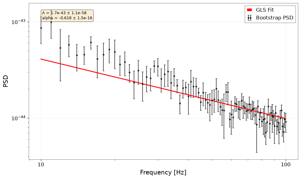
In real analysis, we often estimate the covariance matrix from the data itself using bootstrap methods. GWexpy provides an integrated pipeline for this.

from gwexpy.fitting.highlevel import fit_bootstrap_spectrum
from gwexpy.noise.wave import colored

# Generate 10 seconds of pink noise
data = colored(duration=10, sample_rate=256, exponent=0.5, amplitude=1e-21)

def power_law(f, A, alpha):
    return A * f**alpha

result = fit_bootstrap_spectrum(
    data,
    model_fn=power_law,
    freq_range=(10, 100),
    fftlength=1.0,
    overlap=0.5,
    initial_params={"A": 1e-21, "alpha": -0.5},
    plot=True
)

4. Exercises

1. Parameter Bounds: Modify the OLS fit to restrict A > 0 using the limits argument in fit_series.

2. MCMC: Enable MCMC in Section 3 by setting run_mcmc=True (requires emcee).

5. Quick Check (NBMAKE)

assert "A" in res.params
assert result.reduced_chi2 > 0
print("Validation successful!")

Validation successful!