Development documentation · 0.2.3 30c2f8ba · Intro examples tested with 0.2.3 · Version details · Known limitations

Noise Generation: Basics

Goal: Learn how to generate, manipulate, and model noise in gravitational-wave data using GWexpy.

Prerequisites:

• gwinc (optional, for detector models)

• obspy (optional, for seismic models)

From an ASD model to a measured spectrum

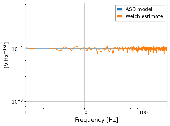
This first example needs only the base installation. The model is a one-sided voltage ASD, not a sample standard deviation. A fixed seed makes the generated waveform reproducible. Welch averaging estimates the model with finite statistical scatter; individual bins need not equal the model.

from astropy import units as u
from gwexpy.noise import asd
from gwexpy.noise.wave import from_asd
from gwexpy.plot import Plot

model = asd.white_noise(0.01 * u.V / u.Hz**0.5, fmin=0, fmax=256, df=1/16)
waveform = from_asd(model, duration=16, sample_rate=512, seed=42)
measured = waveform.asd(fftlength=2, overlap=1, window="hann", method="welch")
plot = Plot(model, measured, xscale="log", yscale="log")
plot.gca().set_xlim(1, 256)
plot.gca().legend(["ASD model", "Welch estimate"])
plot.savefig("noise-model-comparison.png")
assert measured.unit.is_equivalent(model.unit)

1. Generating ASD (Amplitude Spectral Density)

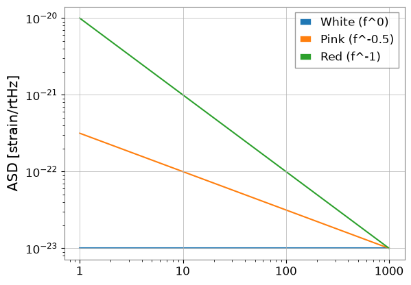
GWexpy provides several ways to generate ASDs, from theoretical power-laws to detector-specific models.

import warnings


import matplotlib.pyplot as plt
import numpy as np

from gwexpy.noise import asd

freqs = np.logspace(0, 3, 1000)

# 1. Power-law ASDs
white = asd.white_noise(amplitude=1e-23, frequencies=freqs)
pink = asd.pink_noise(amplitude=1e-22, f_ref=10, frequencies=freqs)
red = asd.red_noise(amplitude=1e-21, f_ref=10, frequencies=freqs)

plt.loglog(white.xindex, white, label="White (f^0)")
plt.loglog(pink.xindex, pink, label="Pink (f^-0.5)")
plt.loglog(red.xindex, red, label="Red (f^-1)")
plt.ylabel("ASD [strain/rtHz]")
plt.legend()
plt.show()

2. Generating Time-domain Noise

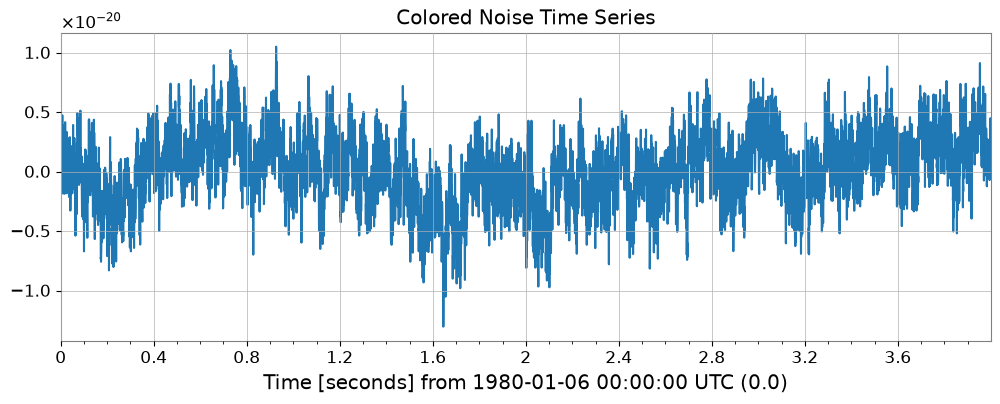
You can generate colored noise directly in the time domain using gwexpy.noise.wave.

from gwexpy.noise import wave

duration = 4.0
fs = 2048

# Generate pink noise time series
noise_ts = wave.pink_noise(duration=duration, sample_rate=fs, amplitude=1e-21)

noise_ts.plot()
plt.title("Colored Noise Time Series")
plt.show()

3. Spectral Lines and Masking

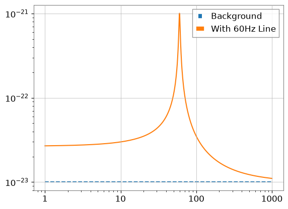
Real noise contains narrow resonance peaks (lines). You can add them using Lorentzian or Gaussian shapes.

from gwexpy.noise.asd import lorentzian_line

# lorentzian_line requires Q or gamma (HWHM)
line = lorentzian_line(f0=60, gamma=1.0, amplitude=1e-21, frequencies=freqs)
total_asd = white + line

plt.loglog(freqs, white.value, "--", label="Background")
plt.loglog(freqs, total_asd.value, label="With 60Hz Line")
plt.legend()
plt.show()

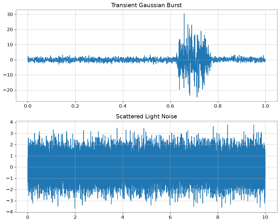
4. Non-Gaussian Noise (Glitches)

gwexpy.noise.non_gaussian provides models for non-stationary noise like scattered light or transient bursts.

from gwexpy.noise.non_gaussian import scatter_light_noise, transient_gaussian_noise

# 1. Transient burst (Model I)
burst = transient_gaussian_noise(duration=1.0, sample_rate=fs, A1=10.0)

# 2. Scattered light (Model II)
scatter = scatter_light_noise(duration=10.0, sample_rate=fs, A2=1e-6, G=1e-21)

fig, ax = plt.subplots(2, 1, figsize=(10, 8))
ax[0].plot(burst.times, burst); ax[0].set_title("Transient Gaussian Burst")
ax[1].plot(scatter.times, scatter); ax[1].set_title("Scattered Light Noise")
plt.tight_layout()
plt.show()

5. Case Study: Simple Noise Budget

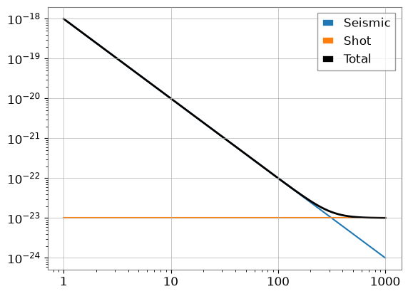
Combine multiple noise sources (seismic, thermal, shot noise) to create a total noise budget.

# seismic ~ f^-2
seismic = asd.power_law(exponent=2, amplitude=1e-20, f_ref=10, frequencies=freqs)
# shot ~ f^0
shot = asd.white_noise(amplitude=1e-23, frequencies=freqs)

total = np.sqrt(seismic.value**2 + shot.value**2)

plt.loglog(freqs, seismic.value, label="Seismic")
plt.loglog(freqs, shot.value, label="Shot")
plt.loglog(freqs, total, "k", lw=2, label="Total")
plt.legend()
plt.show()

Common Mistakes and Failure Modes

• Assuming the ASD slope alone validates the time-domain realization: a generated noise series can match the target trend on average while still differing in finite-length variance, line structure, or transient content.

• Reading synthetic components as independent just because they were generated separately: when you combine seismic, thermal, and shot-noise-like terms, the total curve is a modeling construction, not evidence that real detector subsystems are separable that way.

• Confusing line amplitude with line width or quality factor: for narrow spectral features, changing Q or gamma affects interpretation differently from changing overall amplitude.

• Over-interpreting glitches as realistic populations: the non-Gaussian examples illustrate shapes and workflow behavior, not a calibrated model of real glitch rates or detector environments.

• Comparing curves without checking units and reference frequencies: a visually reasonable power law can still be mis-parameterized if amplitude, exponent, or f_ref are interpreted inconsistently.

• Treating a simple noise budget as a validated instrument budget: the case study shows how to combine terms numerically, but it is not a substitute for validated coupling measurements or full uncertainty accounting.

6. Exercises

1. Spectrum-to-Time: Use wave.colored to generate a 10-second signal with an exponent of 1.5, then plot its ASD to verify the slope.

2. Line Removal: (Challenge) Remove the 60Hz line generated in Section 3.

7. Quick Check Cell (NBMAKE)

Used for automated CI validation.

assert len(white) == 1000
assert noise_ts.sample_rate.value == 2048
print("Validation successful!")

Validation successful!