Development documentation · 0.2.3 30c2f8ba · Intro examples tested with 0.2.3 · Version details · Known limitations

Quickstart#

Create two synthetic channels, calculate their amplitude spectral densities (ASDs), and save asd.png. Prerequisites: Python 3.11 or later and GWexpy installed; no detector files or optional packages are needed. Study goal: about 5 minutes after installation. Script runtime goal: seconds on a laptop; this is not a benchmark.

Install GWexpy#

In a terminal with your chosen Python environment active, run:

python -m pip install gwexpy

For environment creation and Conda instructions, use Installation.

Run the complete example#

Download quickstart.py into a working folder and run the command below from that folder. A terminal command starts Python; the downloaded file contains the Python statements it will execute in order.

python quickstart.py

"""Generate two synthetic channels and save their ASDs to asd.png."""

# quickstart-begin
from gwexpy.noise.wave import gaussian, sine
from gwexpy.timeseries import TimeSeriesDict

settings = dict(duration=16, sample_rate=512, t0=0, unit="V")
tone = sine(frequency=40, **settings)
channels = TimeSeriesDict(
    {
        "Sensor A": tone + gaussian(std=0.3, seed=10, **settings),
        "Sensor B": tone + gaussian(std=0.8, seed=20, **settings),
    }
)
spectra = channels.asd(fftlength=2, overlap=1, window="hann", method="welch")
plot = spectra.plot(xlim=(1, 256), ylabel=r"ASD [V/$\sqrt{\mathrm{Hz}}$]")
plot.gca().legend()
plot.savefig("asd.png")
# quickstart-end

The sine and gaussian functions create TimeSeries objects with the same 16-second duration, 512 Hz sample rate, start time, and volt unit. Explicit seeds make both noise sequences repeatable. TimeSeriesDict keeps the two named channels together, and .asd() applies the same spectral settings to each one. The final line saves the figure in the folder where the command runs; open asd.png with an image viewer.

Read the result#

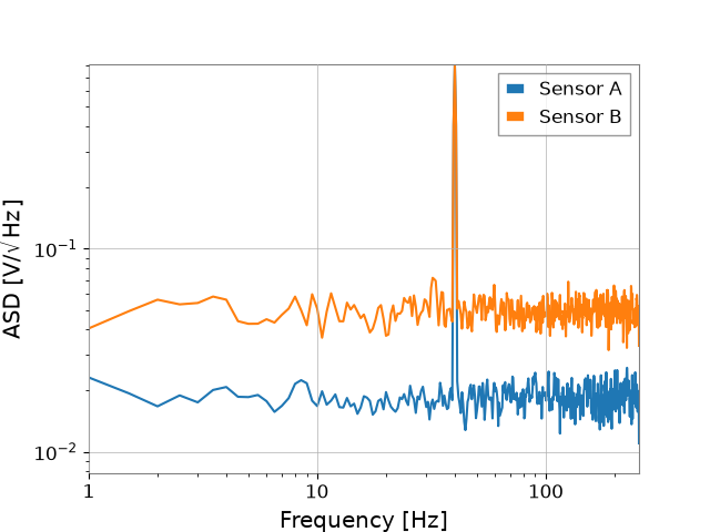
Two voltage amplitude spectral densities with a shared peak near 40 Hz and different noise floors. — Expected output from the downloadable example: a 40 Hz line in both channels and a higher broadband noise floor in Sensor B.#

The horizontal axis is frequency in hertz; the vertical axis is ASD in volts per square root hertz. An ASD shows how fluctuation amplitude is distributed over frequency. Both channels contain the same 40 Hz sine wave, while Sensor B has larger Gaussian noise. The peak height also depends on the spectral settings; it is not the sine wave’s amplitude in volts.

fftlength=2 uses 2-second segments, giving a frequency-bin spacing of 0.5 Hz. overlap=1 overlaps adjacent segments by 1 second. The example explicitly selects a Hann window and Welch averaging so the analysis choices are visible.

Change one parameter#

Change frequency=40 to frequency=70 and run the script again. The two peaks should move to 70 Hz. Then restore 40 Hz and try changing one noise standard deviation (std) to see how the broadband floor responds.

If the script does not run#

ModuleNotFoundError: No module named 'gwexpy' means the Python running the script cannot find GWexpy. Activate the environment used for installation, then rerun python quickstart.py. For other symptoms, use Troubleshooting.