
TimeSeries: Basics#
Create a voltage signal, inspect its metadata, select an interval, and save a plot. Prerequisites: the Quickstart. No optional analysis packages or external data are needed. Allow about 15 minutes to read and run the lesson.
1. Create a signal#
This is the same 40 Hz tone and seeded sensor noise used in the Quickstart.
A TimeSeries keeps sample values together with their unit, start time, and cadence.
from gwexpy.noise.wave import gaussian, sine

settings = dict(duration=16, sample_rate=512, t0=0, unit="V")
signal = sine(frequency=40, **settings) + gaussian(std=0.3, seed=10, **settings)
signal.name = "Sensor A"
2. Inspect values and metadata#
value contains an array of sample values; unit, t0, and sample_rate explain
what those numbers mean. dt is the time between samples. Keep these attributes
when exporting values to another tool.
print(signal[:5])
print("Unit:", signal.unit)
print("Start:", signal.t0)
print("Sample rate:", signal.sample_rate)
print("Cadence:", signal.dt)
assert signal.size == 16 * 512
TimeSeries([-0.33100153,  0.25388934,  0.59692804,  1.07527748,
             0.84930531],
           unit: V,
           t0: 0.0 s,
           dt: 0.001953125 s,
           name: Sensor A,
           channel: None)
Unit: V
Start: 0.0 s
Sample rate: 512.0 Hz
Cadence: 0.001953125 s
3. Select an interval#
The interval starts at 2 seconds and ends just before 4 seconds. Assign the
returned series to a new name so the full input remains available. For a
TimeSeriesDict, use channels.copy().crop(...) to preserve the collection.
segment = signal.crop(2, 4, copy=True)
assert segment.size == 2 * 512
assert signal.size == 16 * 512
4. Plot and save#
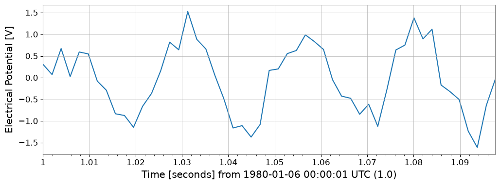
A short interval makes individual oscillations visible. The plot labels the
sample unit, and savefig writes a figure that can be used in a log or slide.
plot = signal.crop(2, 2.1, copy=True).plot()
plot.savefig("timeseries.png")
5. Estimate an ASD#
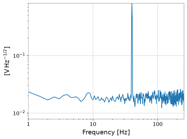
Use the full 16-second record for averaging. Two-second Hann-windowed segments with one-second overlap give 0.5 Hz frequency bins. ASD is expressed in V per square root Hz; it is not the amplitude of an individual sine wave.
spectrum = signal.asd(fftlength=2, overlap=1, window="hann", method="welch")
plot = spectrum.plot(xlim=(1, 256))
plot.savefig("timeseries-asd.png")
assert spectrum.unit.is_equivalent(signal.unit / signal.sample_rate.unit**0.5)
Next lessons#
Commissioner: read channels, compare ASD and coherence, and save conditions.
Noise generation: create a spectral model and compare it with measured noise.
Spectral analysis: time-frequency methods and peak detection.
Lock-in detection: demodulation with known references.
HHT, ARIMA, and interoperability cover the former advanced sections.