Note
このページは Jupyter Notebook から生成されました。 ノートブックをダウンロード (.ipynb)
[1]:
# Skipped in CI: Colab/bootstrap dependency install cell.
ARIMA: 時系列予測
![]()
このノートブックでは、gwexpy の TimeSeries クラスに追加された ARIMA 関連の機能(AR, MA, ARMA, ARIMA/SARIMAX)を使用して、時系列データのモデリングと未来予測を行う方法を解説します。
関連 API: Time Series API
関連理論: 検証済みアルゴリズム, 数値安定性
準備
必要なライブラリをインポートします。
[2]:
import warnings

import matplotlib.pyplot as plt
import numpy as np
import sklearn.utils.validation

# Monkeypatch for pmdarima compatibility with scikit-learn >= 1.6
_orig_check_array = sklearn.utils.validation.check_array

def _patched_check_array(*args, **kwargs):
    kwargs.pop("force_all_finite", None)
    return _orig_check_array(*args, **kwargs)

sklearn.utils.validation.check_array = _patched_check_array

warnings.filterwarnings(
    "ignore", message=r".*force_all_finite.*", category=FutureWarning
)
warnings.filterwarnings("ignore", category=FutureWarning, module=r"sklearn\..*")
warnings.filterwarnings("ignore", category=FutureWarning, module=r"pmdarima\..*")

from gwexpy.timeseries import TimeSeries
サンプルデータの作成
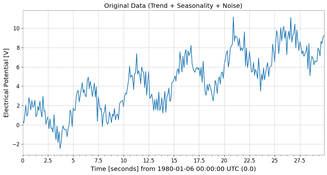
ARIMAモデルの効果を確認するために、トレンド、季節性(周期性)、ノイズを含んだ模擬データを作成します。
[3]:
# Trend + Seasonality + Noise
t0 = 0
dt = 0.1
duration = 30
t = np.arange(0, duration, dt)
n_samples = len(t)

# 1. Linear Trend
trend = 0.3 * t

# 2. Periodic component (Sine)
seasonality = 2.0 * np.sin(2 * np.pi * 0.2 * t)

# 3. Noise
np.random.seed(42)
noise = np.random.normal(0, 0.8, n_samples)

data = trend + seasonality + noise

# Create TimeSeries object
ts = TimeSeries(data, t0=t0, dt=dt, unit="V", name="Sample Data")

ts.plot()
plt.title("Original Data (Trend + Seasonality + Noise)")
plt.show()
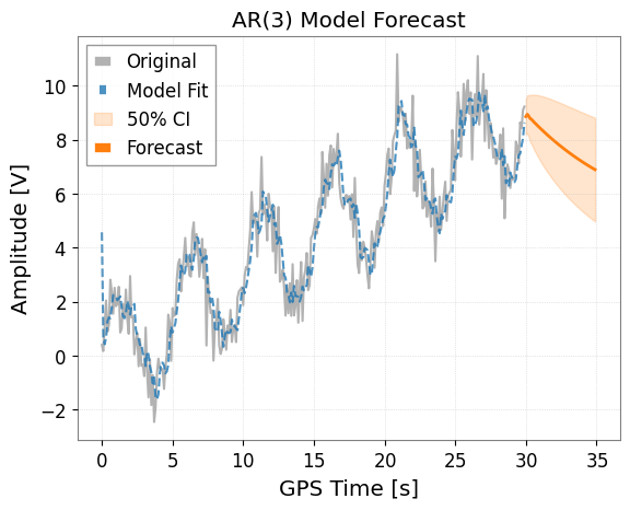
1. AR (AutoRegressive) モデル
ARモデルは、現在の値が過去の値に依存すると仮定するモデルです。 ts.ar(p) メソッドを使用します。p は次数です。
[4]:
# Fit with order p=3
model_ar = ts.ar(p=3)

# Display model summary
# print(model_ar.summary())

# Plot results
# forecast_steps specifies how many steps to forecast into the future
model_ar.plot(forecast_steps=50, alpha=0.5)
plt.title("AR(3) Model Forecast")
plt.show()
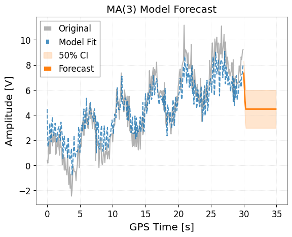
2. MA (Moving Average) モデル
MAモデルは、現在の値が過去の予測誤差(ホワイトノイズ)に依存すると仮定するモデルです。 ts.ma(q) メソッドを使用します。
[5]:
# Fit with order q=3
model_ma = ts.ma(q=3)

# Plot results
model_ma.plot(forecast_steps=50, alpha=0.5)
plt.title("MA(3) Model Forecast")
plt.show()
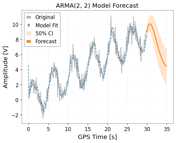
3. ARMA (AutoRegressive Moving Average) モデル
ARとMAを組み合わせたモデルです。 ts.arma(p, q) メソッドを使用します。
[6]:
# Fit with p=2, q=2
model_arma = ts.arma(p=2, q=2)

model_arma.plot(forecast_steps=50, alpha=0.5)
plt.title("ARMA(2, 2) Model Forecast")
plt.show()
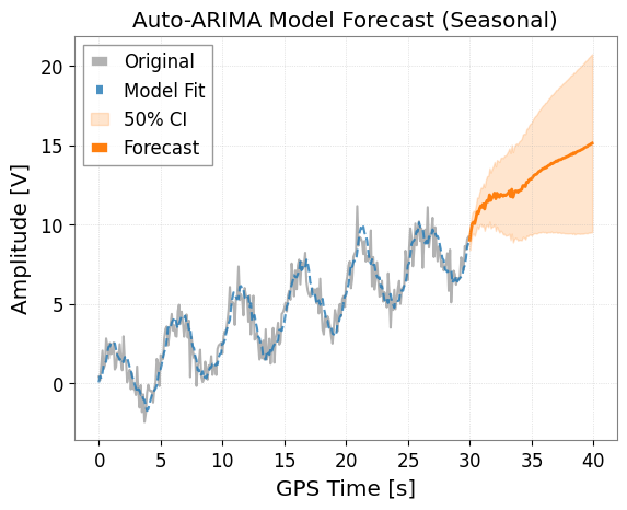
4. ARIMA / Auto-ARIMA
ARIMAモデルは、差分を取ることで非定常性(トレンドなど)を除去し、ARMAモデルを適用します。
ts.arima() メソッドを使用します。 auto=True オプションを指定すると、pmdarima ライブラリを使用して最適なパラメータ (p, d, q) を自動的に探索します。これが最も推奨される方法です。
[7]:
try:
    print("Searching for optimal ARIMA parameters... (this may take a few seconds)")

    # Seasonality can also be considered
    # m is the number of steps in a seasonal period
    model_auto = ts.arima(auto=True, auto_kwargs={"seasonal": True, "m": 50})

    # Show info of the optimal model found
    print(model_auto.summary())

    # Plot results (Forecasting for a longer period)
    ax = model_auto.plot(forecast_steps=100, alpha=0.5)
    plt.title("Auto-ARIMA Model Forecast (Seasonal)")
    plt.show()
except ImportError as e:
    print(f"Auto-ARIMA skipping: {e}")
Searching for optimal ARIMA parameters... (this may take a few seconds)
                                      SARIMAX Results
===========================================================================================
Dep. Variable:                                   y   No. Observations:                  300
Model:             SARIMAX(1, 1, 2)x(1, 0, [], 50)   Log Likelihood                -404.141
Date:                             Sun, 05 Jul 2026   AIC                            820.282
Time:                                     15:45:01   BIC                            842.485
Sample:                                          0   HQIC                           829.169
                                             - 300
Covariance Type:                               opg
==============================================================================
                 coef    std err          z      P>|z|      [0.025      0.975]
------------------------------------------------------------------------------
intercept      0.0044      0.006      0.695      0.487      -0.008       0.017
ar.L1          0.8693      0.053     16.310      0.000       0.765       0.974
ma.L1         -1.6277      0.052    -31.464      0.000      -1.729      -1.526
ma.L2          0.7409      0.043     17.235      0.000       0.657       0.825
ar.S.L50       0.1604      0.071      2.263      0.024       0.021       0.299
sigma2         0.8667      0.070     12.431      0.000       0.730       1.003
===================================================================================
Ljung-Box (L1) (Q):                   0.13   Jarque-Bera (JB):                 0.69
Prob(Q):                              0.71   Prob(JB):                         0.71
Heteroskedasticity (H):               1.37   Skew:                            -0.10
Prob(H) (two-sided):                  0.12   Kurtosis:                         3.14
===================================================================================

Warnings:
[1] Covariance matrix calculated using the outer product of gradients (complex-step).
5. 予測データの取得
プロットだけでなく、.forecast() メソッドを使用して予測値の TimeSeries オブジェクトを直接取得できます。 これには信頼区間(Confidence Interval)も含まれます。
[8]:
if "model_auto" not in dir():
    print("Auto-ARIMA model not available (pmdarima may be missing); skipping forecast.")
else:
    steps = 50

    # Get forecast values and confidence intervals
    forecast_ts, intervals = model_auto.forecast(
        steps=steps, alpha=0.5
    )  # 50% confidence interval

    print("Forecast Data:")
    print(forecast_ts)

    print("\nConfidence Interval (Upper):")
    print(intervals["upper"])

    # Forecasting data can be saved or used for other analysis
    # forecast_ts.write("forecast.h5")
Forecast Data:
TimeSeries([ 9.02062915,  9.60946405, 10.04247456, 10.15366445,
            10.052592  , 10.38952912, 10.79814617, 10.71027098,
            11.00660121, 11.18204481, 11.08229647, 11.29882151,
            10.98338727, 11.34915911, 11.51884639, 11.45194911,
            11.87326351, 11.52377866, 11.68682442, 11.7893815 ,
            11.9809718 , 11.6301489 , 11.97772171, 11.84041478,
            11.72114873, 11.91253389, 11.8838869 , 11.78615925,
            11.8774296 , 11.82550574, 11.89782592, 11.97898836,
            12.11131514, 11.7662658 , 12.22000645, 11.72132856,
            11.98238211, 12.11214327, 12.11235985, 12.04093447,
            12.14348261, 12.16096473, 12.20710207, 12.45441741,
            12.45770285, 12.39286443, 12.6699954 , 12.66916833,
            12.81102595, 12.86571835],
           unit: V,
           t0: 30.0 s,
           dt: 0.1 s,
           name: Sample Data_auto_forecast,
           channel: None)

Confidence Interval (Upper):
TimeSeries([ 9.64857072, 10.2554647 , 10.71958565, 10.87455716,
            10.82818047, 11.22843787, 11.70674543, 11.69298419,
            12.06628628, 12.32035105, 12.29996294, 12.59591292,
            12.35947544, 12.80346063, 13.05032641, 13.05939929,
            13.55536057, 13.27912824, 13.51399385, 13.68692426,
            13.94744559, 13.66412891, 14.07781018, 14.00524778,
            13.94940078, 14.20292097, 14.23516817, 14.19713784,
            14.34695277, 14.35246436, 14.4811537 , 14.61766074,
            14.80434796, 14.51271392, 15.01896222, 14.57192023,
            14.88377233, 15.06352749, 15.11296484, 15.0900168 ,
            15.2403272 , 15.3048835 , 15.39743258, 15.69052159,
            15.7389658 , 15.71869326, 16.03981815, 16.0824329 ,
            16.26719914, 16.36428493],
           unit: V,
           t0: 30.0 s,
           dt: 0.1 s,
           name: upper_ci,
           channel: None)
6. 重力波データ解析における応用: ARIMAによるノイズ除去 (Whitening)
重力波データ解析では、定常的な「有色ノイズ」の中から突発的なバースト信号やリングダウン波形を抽出するために、白色化 (Whitening) という処理が行われます。 ARIMAモデルを背景ノイズの予測モデルとして学習させ、実測値からその予測値を引く(残差をとる)ことで、ノイズを除去し信号を強調することが可能です。
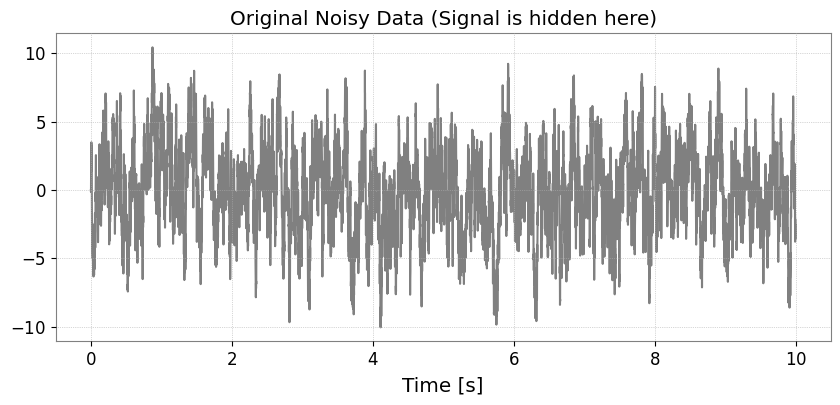
Step 1: 有色ノイズの生成と信号の注入
まず、低周波成分が強い有色ノイズ(AR(1)プロセス)を作成し、そこにそのままでは判別しにくい微弱な信号(サインガウシアン)を埋め込みます。 ※単位には Astropy で認識可能な “strain” を使用します。
[9]:
import matplotlib.pyplot as plt
import numpy as np

from gwexpy.timeseries import TimeSeries


def generate_mock_data(duration=10, fs=1024):
    t = np.linspace(0, duration, int(duration * fs))

    # 1. Background Noise (AR(1) process with strong autocorrelation)
    np.random.seed(42)
    white_noise = np.random.normal(0, 1, len(t))
    colored_noise = np.zeros_like(white_noise)
    for i in range(1, len(t)):
        colored_noise[i] = 0.95 * colored_noise[i - 1] + white_noise[i]

    # 2. Injected Signal (Sine-Gaussian)
    center_time = 5.0
    sig_freq = 50.0
    width = 0.1
    signal = (
        2.0
        * np.exp(-((t - center_time) ** 2) / (2 * width**2))
        * np.sin(2 * np.pi * sig_freq * t)
    )

    data = colored_noise + signal
    # Use a standard unit string that astropy/gwpy can recognize
    return TimeSeries(data, t0=0, dt=1 / fs, unit="strain", name="MockData")


ts = generate_mock_data()

plt.figure(figsize=(10, 4))
plt.plot(ts, color="gray")
plt.title("Original Noisy Data (Signal is hidden here)")
plt.xlabel("Time [s]")
plt.grid(True, linestyle=":")
plt.show()
Step 2: ARIMAによるノイズモデリング
auto=True を使って、背景ノイズの自己相関構造を表現する最適なモデルを探索します。
[10]:
print("Searching for optimal noise model parameters...")
# We prioritize AR model for whitening, so we set max_p=5 and max_q=0.
model = ts.arima(auto=True, max_p=5, max_q=0)
print(f"Best model order: {model.res.model.order}")
print(model.summary())
Searching for optimal noise model parameters...
Best model order: (5, 1, 0)
                               SARIMAX Results
==============================================================================
Dep. Variable:                      y   No. Observations:                10240
Model:               SARIMAX(5, 1, 0)   Log Likelihood              -14694.968
Date:                Sun, 05 Jul 2026   AIC                          29403.936
Time:                        15:45:13   BIC                          29454.574
Sample:                             0   HQIC                         29421.057
                              - 10240
Covariance Type:                  opg
==============================================================================
                 coef    std err          z      P>|z|      [0.025      0.975]
------------------------------------------------------------------------------
intercept     -0.0003      0.010     -0.033      0.973      -0.020       0.019
ar.L1         -0.0379      0.010     -3.794      0.000      -0.057      -0.018
ar.L2         -0.0413      0.010     -4.150      0.000      -0.061      -0.022
ar.L3         -0.0271      0.010     -2.692      0.007      -0.047      -0.007
ar.L4         -0.0303      0.010     -3.078      0.002      -0.050      -0.011
ar.L5         -0.0216      0.010     -2.195      0.028      -0.041      -0.002
sigma2         1.0330      0.014     72.089      0.000       1.005       1.061
===================================================================================
Ljung-Box (L1) (Q):                   0.01   Jarque-Bera (JB):                 0.54
Prob(Q):                              0.94   Prob(JB):                         0.76
Heteroskedasticity (H):               1.03   Skew:                             0.01
Prob(H) (two-sided):                  0.35   Kurtosis:                         3.03
===================================================================================

Warnings:
[1] Covariance matrix calculated using the outer product of gradients (complex-step).
Step 3: 残差(Residuals)の抽出と可視化
モデルが予測した「定常ノイズ」を引くことで、残差 \(x_r = x - \hat{x}\) を求めます。これが白色化されたデータとなります。
[11]:
ts_whitened = model.residuals()
ts_whitened.name = "Whitened Data"

fig, ax = plt.subplots(2, 1, figsize=(10, 8), sharex=True)

ax[0].plot(ts, color="gray", alpha=0.5, label="Original")
ax[0].set_title("Original Noisy Data")
ax[0].legend(loc="upper right")

ax[1].plot(ts_whitened, color="red", label="Residuals (Whitened)")
ax[1].set_title("Whitened Data (Signal is now visible!)")
ax[1].axvspan(4.8, 5.2, color="orange", alpha=0.3, label="Injected Signal Position")
ax[1].legend(loc="upper right")

plt.tight_layout()
plt.show()

Step 4: 周波数領域での評価
パワースペクトル密度 (PSD) を計算して比較します。
[12]:
fft_original = ts.psd()
fft_whitened = ts_whitened.psd()

plt.figure(figsize=(10, 5))
plt.loglog(
    fft_original.frequencies.value,
    fft_original.value,
    label="Original Noisy PSD",
    alpha=0.7,
)
plt.loglog(
    fft_whitened.frequencies.value,
    fft_whitened.value,
    label="Whitened PSD (Residuals)",
    alpha=0.7,
)
plt.title("PSD Comparison: Effect of ARIMA Whitening")
plt.xlabel("Frequency [Hz]")
plt.ylabel("PSD [1/Hz]")
plt.legend()
plt.grid(True, which="both", linestyle=":")
plt.show()
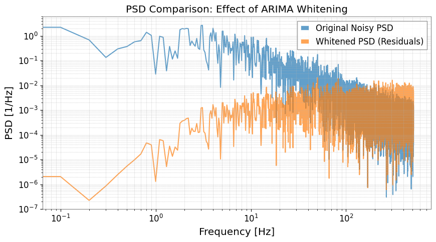
まとめ
model.residuals()を用いることで、複雑な数式を書かずに簡単に白色化処理が実行できます。この手法は、重力波解析におけるバースト信号の探索や、イベント直後のリングダウン波形(指数減衰する正弦波)の抽出に非常に強力です。
関連 API: Time Series API
関連理論: 検証済みアルゴリズム, 数値安定性