Note
This page was generated from a Jupyter Notebook. Download the notebook (.ipynb)
[1]:
# Skipped in CI: Colab/bootstrap dependency install cell.
Bruco: Basics
![]()
Bruco is a tool for computing “Brute force coherence”. It calculates the coherence between the main channel (target) of gravitational wave detectors (LIGO or Virgo) and numerous auxiliary channels to identify noise sources. Physically, the goal is not just to rank channels, but to test whether a witness can plausibly explain excess DARM power in a specific frequency band and therefore point to an actionable coupling path.
Coherence Calculation with Parallel Processing
Parallel execution is performed across multiple CPU cores using Python’s multiprocessing module.
Task Division: The entire auxiliary channel list is divided according to the number of CPUs and assigned to each process.
Data Acquisition and Preprocessing:
Acquire data for each auxiliary channel.
Skip if the data is constant (flat).
If the sampling rate is higher than the output request rate (
outfs), downsample using thedecimatefunction.
Coherence Calculation:
Calculate the FFT and PSD (Power Spectral Density) of the auxiliary channel.
Calculate the CSD (Cross Spectral Density) with the target channel.
Calculate the coherence using the following formula:
Selection of Top N:
For all frequency bins, if the calculated coherence value is higher than the existing top list (
top), update the value. This efficiently records only the highly correlated top channels instead of keeping results for all channels.
Result Aggregation and Output:
Combine and sort
cohtab(coherence values) andidxtab(channel IDs) returned from each process to create the final top list.HTML Report Generation: Use
markup.pyto generateindex.html. This includes tables of top correlated channels for each frequency (with heatmap-style coloring) and links to plot images.Plot Generation: Use
matplotlibto generate coherence and spectrum graphs (PNG or PDF).
This implementation is characterized by the use of pre-computed FFTs, parallel processing, and a memory-efficient Top-N recording method to efficiently process large amounts of channel data.
The original Bruco implementation is available at:
Refer to this for design details and CLI behavior.
This notebook demonstrates the advantages of using the gwexpy Bruco module as a Python library by showing interactive analysis, flexible data manipulation, and advanced hypothesis testing.
We do not use real data, but instead utilize pseudo-data generated with
gwpy/numpy.We demonstrate rapid hypothesis testing for “nonlinear coupling” and “modulation” scenarios that are difficult with the CLI, using the Python API.
Common mistake: interpreting a large coherence peak as proof of causal coupling. Coherence is a ranking tool, not a proof. Before acting on a channel, verify that the witness is physically upstream of DARM, check for common drivers, and confirm that the feature survives reasonable changes in windowing, preprocessing, and segment choice.
Setup and Mock Data Generation
What we do: Create pseudo-data for target/auxiliary channels and prepare TimeSeries to feed into Bruco. Why it’s important: In actual operations, data is acquired from NDS or frames, but being able to freely design signals in a notebook accelerates hypothesis testing.
[2]:
import warnings
warnings.filterwarnings("ignore", category=UserWarning)
warnings.filterwarnings("ignore", category=DeprecationWarning)

# ruff: noqa: I001
from astropy import units as u
import matplotlib.pyplot as plt
import numpy as np

from gwexpy.analysis import Bruco
from gwexpy.analysis.bruco import FastCoherenceEngine
from gwexpy.astro import inspiral_range
from gwexpy.frequencyseries import FrequencySeriesDict
from gwexpy.noise.asd import from_pygwinc
from gwexpy.noise.wave import from_asd
from gwexpy.plot import Plot
from gwexpy.timeseries import TimeSeries, TimeSeriesDict
[3]:
rng = np.random.default_rng(7)
duration = 128 # seconds
sample_rate = 2048 # Hz
fftlength = 4.0 # seconds
overlap = 2.0 # seconds
t = np.arange(0, duration, 1 / sample_rate)
# Get aLIGO sensitivity curve (ASD)
fmax = sample_rate / 2 # Nyquist frequency
asd_aligo = from_pygwinc(
"aLIGO", fmin=4.0, fmax=fmax, df=1.0 / duration, quantity="strain"
)
# Generate target noise based on aLIGO sensitivity curve
target = from_asd(asd_aligo, duration, sample_rate, t0=0, rng=rng).highpass(1)
target.channel = "H1:TARGET"
# Signals for auxiliary channels
fast_line = np.sin(2 * np.pi * 60.0 * t)
slow_motion = 70 * np.sin(2 * np.pi * 2.3 * t) + 30 * np.sin(2 * np.pi * 7.1 * t)
aux1_data = 0.8 * fast_line + 0.2 * rng.normal(0, 1.0, size=t.size)
aux2_data = 0.9 * slow_motion + 0.2 * rng.normal(0, 1.0, size=t.size) + 1
aux1 = TimeSeries(
aux1_data, sample_rate=sample_rate, t0=0, unit="V", channel="H1:AUX1_FAST"
)
aux2 = TimeSeries(
aux2_data, sample_rate=sample_rate, t0=0, unit="V", channel="H1:AUX2_SLOW"
).lowpass(30)
# Injection signal into target: aLIGO-based noise + linear coupling + nonlinear injection
target = target + 1e-22 * target.unit * (
aux1 / u.V + aux2 / u.V + (aux1 / u.V / 2) ** 2 + 0.01 * (aux1 * aux2 / u.V**2)
)
target.name = target.channel
aux1.name = aux1.channel
aux2.name = aux2.channel
aux_dict = TimeSeriesDict(
{
aux1.channel: aux1,
aux2.channel: aux2,
}
)
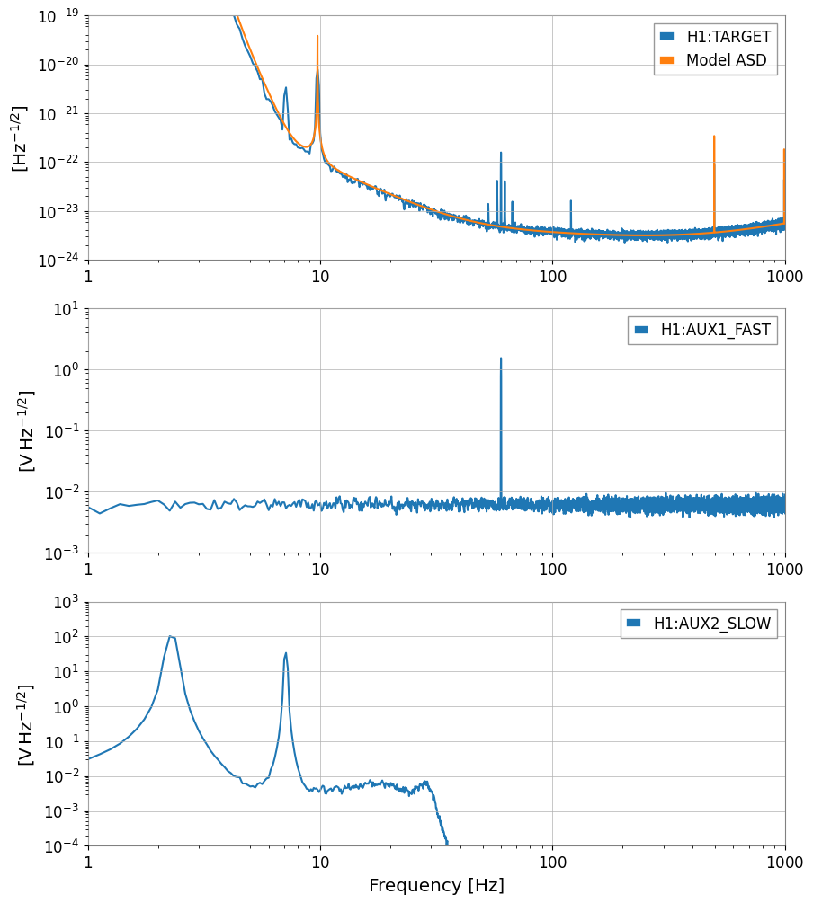
print(f"aLIGO ASD at 100 Hz: {asd_aligo.crop(99, 101).value[0]:.2e} strain/sqrt(Hz)")
print(f"Target data std: {target.std():.2e}")
plot = Plot(
[target.asd(8, 4), asd_aligo],
aux1.asd(8, 4),
aux2.asd(8, 4),
figsize=(10, 12),
sharex=True,
)
axes = plot.get_axes()
axes[0].set_xlim(1, 1e3)
axes[0].set_ylim(1e-24, 1e-19)
axes[1].set_ylim(1e-3, 1e1)
axes[2].set_ylim(1e-4, 1e3)
axes[0].legend([target.name, "Model ASD"])
axes[1].legend([aux1.name])
axes[2].legend([aux2.name])
aLIGO ASD at 100 Hz: 3.71e-24 strain/sqrt(Hz)
Target data std: 5.08e-19
[3]:
<matplotlib.legend.Legend at 0x7f5caab7fcd0>
Section 1: Running Basic Bruco Analysis (Reproduction in Jupyter)
What we do: Run brute force coherence analysis with the Bruco class and verify results with tables and plots. Why it’s important: With the Python API, you can quickly try “culprit searches” while interactively changing conditions and visualizations.
[4]:
# Initialize Bruco.
# Since we manually pass all data here, specify an empty list for auto-fetch channel list (aux_channels).
bruco = Bruco(target_channel=target.name, aux_channels=[])

# By passing target_data and aux_data to the compute method, you can skip internal fetching and run the analysis.
result = bruco.compute(
    start=0,
    duration=int(duration),
    fftlength=fftlength,
    overlap=overlap,
    parallel=1,
    batch_size=2,
    top_n=3,
    target_data=target,  # Pre-generated target data
    aux_data=aux_dict,  # Pre-generated auxiliary channel data dictionary
)
[5]:
df = result.to_dataframe(ranks=[0])

df_sorted = (
    df.sort_values("coherence", ascending=False)
    .dropna(subset=["channel"])
    .head(15)
    .reset_index(drop=True)
)

df_sorted
[5]:
| frequency | rank | channel | coherence | projection | |
|---|---|---|---|---|---|
| 0 | 60.00 | 1 | H1:AUX1_FAST | 0.998699 | 1.118712e-22 |
| 1 | 59.75 | 1 | H1:AUX1_FAST | 0.994909 | 5.587699e-23 |
| 2 | 60.25 | 1 | H1:AUX1_FAST | 0.994519 | 5.570859e-23 |
| 3 | 7.25 | 1 | H1:AUX2_SLOW | 0.973445 | 1.888851e-21 |
| 4 | 7.00 | 1 | H1:AUX2_SLOW | 0.968398 | 2.211076e-21 |
| 5 | 62.25 | 1 | H1:AUX2_SLOW | 0.709532 | 2.210663e-23 |
| 6 | 62.50 | 1 | H1:AUX2_SLOW | 0.695847 | 1.435894e-23 |
| 7 | 7.50 | 1 | H1:AUX2_SLOW | 0.680465 | 2.682833e-22 |
| 8 | 6.75 | 1 | H1:AUX2_SLOW | 0.641778 | 5.413037e-22 |
| 9 | 62.00 | 1 | H1:AUX2_SLOW | 0.615101 | 7.153501e-24 |
| 10 | 131.25 | 1 | H1:AUX1_FAST | 0.482609 | 1.772034e-24 |
| 11 | 203.75 | 1 | H1:AUX1_FAST | 0.471606 | 1.572731e-24 |
| 12 | 57.75 | 1 | H1:AUX2_SLOW | 0.451528 | 1.428494e-23 |
| 13 | 57.50 | 1 | H1:AUX2_SLOW | 0.440484 | 9.442593e-24 |
| 14 | 67.25 | 1 | H1:AUX2_SLOW | 0.430697 | 3.624043e-24 |
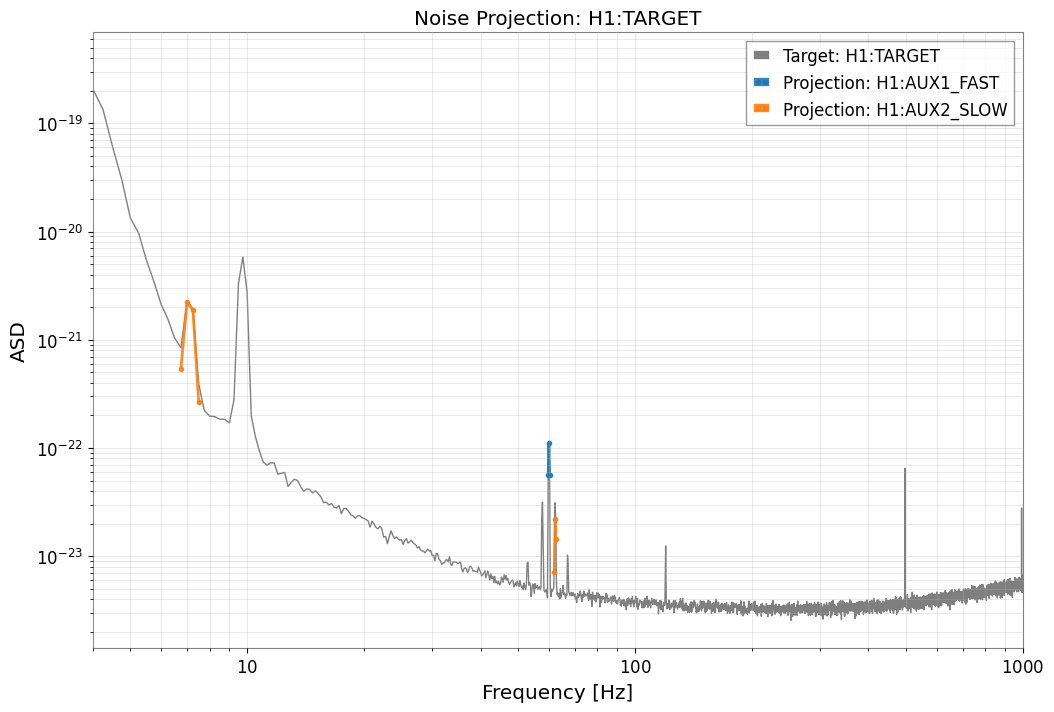
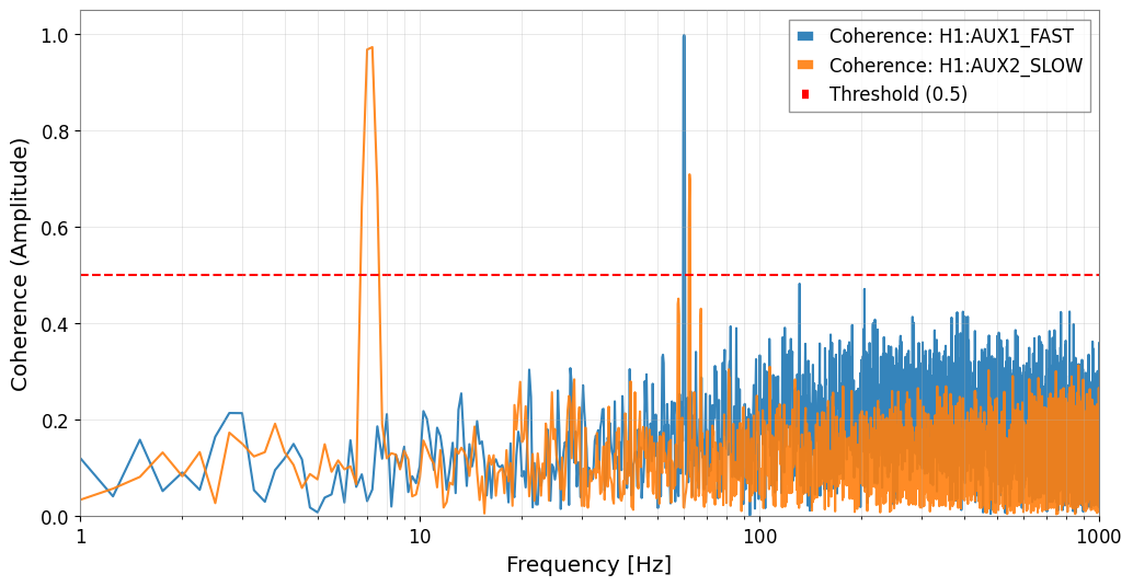
[6]:
result.plot_projection(coherence_threshold=0.5)
plt.xlim(4, 1000)
plt.show()

result.plot_coherence(coherence_threshold=0.5)
plt.xlim(1, 1000)
plt.show()
[7]:
report_path = result.generate_report("bruco_report", coherence_threshold=0.4)
report_path
[7]:
'bruco_report/index.html'
Section 2: Advanced Preprocessing and Hypothesis Testing (Deep Dive: Nonlinear & Bilinear)
What we do: Assume noise that cannot be explained by existing linear correlations and test hypotheses of nonlinear coupling (squared) and modulation (product). Why it’s important: Using FastCoherenceEngine, you can rapidly test virtual channels without recalculating the target FFT.
Physical intent: these virtual channels encode a coupling model such as fast × slow, where a fast carrier is modulated by a slow alignment, control, or environmental drift.
Failure-prone pattern: if you skip the high-pass / band-pass isolation and multiply broadband channels directly, the product is often dominated by irrelevant low-frequency power and the resulting coherence becomes hard to interpret.
Checklist before trusting a virtual witness:
the witness construction matches a plausible coupling mechanism,
the modulation band is narrow enough to be physically meaningful,
the recovered coherence appears where the sidebands or line wandering actually live, not everywhere.
[8]:
ts_sq = aux1**2
ts_sq.name = f"{aux1.name}^2"

ts_prod = aux1 * aux2
ts_prod.name = f"{aux1.name}*{aux2.name}"
[9]:
engine = FastCoherenceEngine(target, fftlength=fftlength, overlap=overlap)

coh_linear = engine.compute_coherence(aux1)
coh_sq = engine.compute_coherence(ts_sq)
coh_prod = engine.compute_coherence(ts_prod)

freqs = engine.frequencies
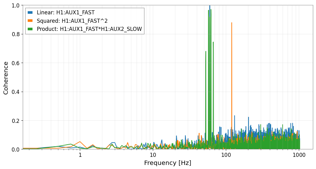
[10]:
fig, ax = plt.subplots(figsize=(12, 6))
ax.semilogx(freqs, coh_linear, label=f"Linear: {aux1.name}")
ax.semilogx(freqs, coh_sq, label=f"Squared: {ts_sq.name}")
ax.semilogx(freqs, coh_prod, label=f"Product: {ts_prod.name}")

ax.set_xlabel("Frequency [Hz]")
ax.set_ylabel("Coherence")
ax.set_ylim(0.0, 1.0)
ax.grid(True, which="both", ls="-", alpha=0.4)
ax.legend()
plt.show()
Section 3: Connection to Downstream Analysis (Actionable Outcome)
What we do: Use the most significant noise hypothesis to estimate the residual spectrum and assess BNS Range improvement. Why it’s important: Rather than stopping at “finding” Bruco results, we can connect them to sensitivity improvement and noise subtraction workflows.
Common mistake: reading the projected residual as a guaranteed subtraction result. The projection assumes the witness is representative and well-conditioned; if the witness is contaminated, delayed, or only intermittently coupled, the predicted improvement can be too optimistic. Treat this section as a screening step before a full subtraction study.
[11]:
target_asd = target.asd(fftlength=fftlength, overlap=overlap)
target_asd_vals = target_asd.value

coh_map = {
    aux1.name: coh_linear,
    ts_sq.name: coh_sq,
    ts_prod.name: coh_prod,
}

dominant_label = max(coh_map, key=lambda k: np.nanmax(coh_map[k]))
dominant_coh = coh_map[dominant_label]

# Estimate virtual channel contribution in ASD using Bruco's projection formula
projected_asd = target_asd_vals * np.sqrt(dominant_coh)
residual_asd_vals = np.sqrt(np.maximum(target_asd_vals**2 - projected_asd**2, 0.0))

residual_asd = target_asd.copy()
residual_asd.value[:] = residual_asd_vals

fig, ax = plt.subplots(figsize=(12, 6))
# ax.loglog(target_asd.frequencies.value, target_asd_vals, label="Target ASD")
# ax.loglog(target_asd.frequencies.value, residual_asd_vals, label="Residual ASD")
ax.loglog(target_asd, label="Target ASD")
ax.loglog(residual_asd, label="Residual ASD")
ax.set_xlabel("Frequency [Hz]")
ax.set_ylabel("ASD")
ax.grid(True, which="both", ls="-", alpha=0.4)
ax.legend()
plt.show()

# BNS Range comparison
bns_range_before = inspiral_range(target_asd**2, mass1=1.4, mass2=1.4, fmin=10)
bns_range_after = inspiral_range(residual_asd**2, mass1=1.4, mass2=1.4, fmin=10)

print(f"Dominant hypothesis: {dominant_label}")
print(f"BNS range (before): {bns_range_before.to_value(u.Mpc):.2f} Mpc")
print(f"BNS range (after):  {bns_range_after.to_value(u.Mpc):.2f} Mpc")
Dominant hypothesis: H1:AUX1_FAST
BNS range (before): 182.48 Mpc
BNS range (after):  186.24 Mpc
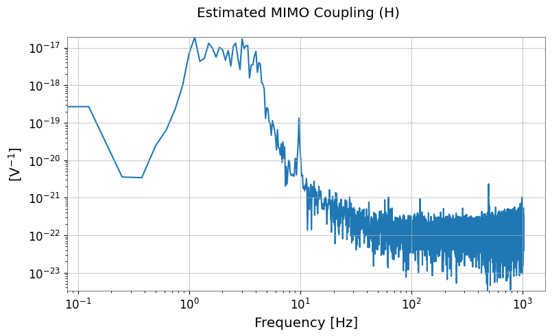
[12]:
virtual_channels = {
aux1.name: aux1,
ts_sq.name: ts_sq,
ts_prod.name: ts_prod,
}
culprit_channels = [dominant_label]
witnesses = TimeSeriesDict({name: virtual_channels[name] for name in culprit_channels})
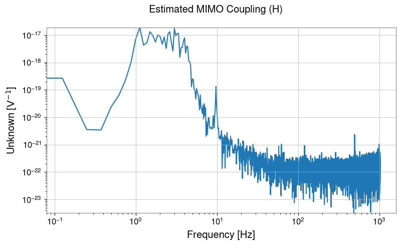
cxx = witnesses.csd_matrix(fftlength=8.0)
cyx = TimeSeriesDict({"TARGET": target}).csd_matrix(other=witnesses, fftlength=8.0)
# Matrix operation H = Cyx @ Cxx^-1
H_lowres = cyx @ cxx.inv()
# Display estimated transfer function
H_lowres.abs().plot(xscale="log", yscale="log").suptitle("Estimated MIMO Coupling (H)")
plt.show()
# Full-resolution FFT
tsd = TimeSeriesDict({"MAIN": target, **witnesses})
aux_names = culprit_channels
tsd_fft = tsd.fft()
main_fft = tsd_fft["MAIN"]
# Filter interpolation and matrix operation
H = H_lowres.interpolate(main_fft.frequencies)
X_mat = FrequencySeriesDict({k: tsd_fft[k] for k in aux_names}).to_matrix()
# Projection and subtraction
Y_proj = (H @ X_mat)[0, 0]
cleaned_fft = main_fft - Y_proj
# To time domain
cleaned_ts = cleaned_fft.ifft()
[13]:
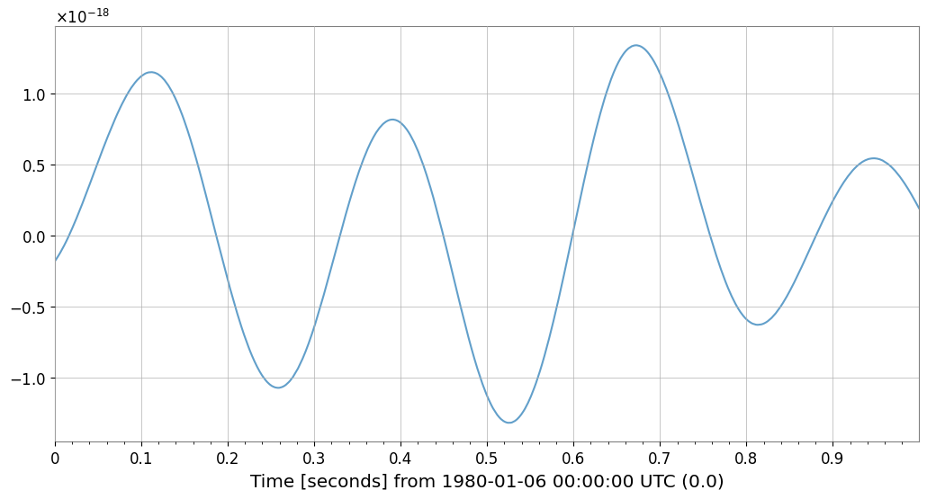
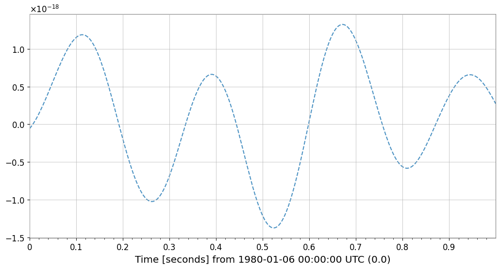
# Verify noise subtraction effect
fig = plt.figure(figsize=(12, 6))
ax = fig.gca()

# Overlay original and cleaned data (first 1 second)
plot_duration = 1.0
target.crop(end=target.t0.value + plot_duration).plot(
    ax=ax, label="Original", alpha=0.7
)  # noqa: F821
cleaned_ts.crop(end=target.t0.value + plot_duration).plot(
    ax=ax, label="Cleaned (Bruco)", linestyle="--", alpha=0.8
)  # noqa: F821

ax.set_title(f"Noise Subtraction Result (First {plot_duration}s)")
ax.legend(["Original", "Cleaned (Bruco)"])
plt.show()