Note

This page was generated from a Jupyter Notebook. Download the notebook (.ipynb)

GWExPy TimeSeries Interoperability Tutorial

This notebook introduces the new interoperability features added to the gwexpy TimeSeries class. gwexpy can seamlessly convert data to and from popular data science libraries such as Pandas, Xarray, PyTorch, and Astropy.

Table of Contents

• 1. General Data Formats & Data Infrastructure

  • 1.1. NumPy [Original GWpy]

  • 1.2. Pandas Integration [Original GWpy]

  • 1.3. Polars [GWExPy New]

  • 1.4. Xarray Integration [Original GWpy]

  • 1.5. Dask Integration [GWExPy New]

  • 1.6. JSON / Python Dict (to_json) [GWExPy New]

• 2. Database & Storage Layer

  • 2.1. HDF5 [Original GWpy]

  • 2.2. SQLite [GWExPy New]

  • 2.3. Zarr [GWExPy New]

  • 2.4. netCDF4 [GWExPy New]

• 3. Computer Science, Machine Learning & Accelerated Computing

  • 3.1. PyTorch Integration [GWExPy New]

  • 3.2. CuPy (CUDA Acceleration) [GWExPy New]

  • 3.3. TensorFlow Integration [GWExPy New]

  • 3.4. JAX Integration [GWExPy New]

• 4. Astronomy & Gravitational Wave Physics

  • 4.1. PyCBC / LAL [Original GWpy]

  • 4.2. Astropy Integration [Original GWpy]

  • 4.3. Specutils Integration [GWExPy New]

  • 4.4. Pyspeckit Integration [GWExPy New]

• 5. Particle Physics & High Energy Physics

  • 5.1. CERN ROOT Integration [GWExPy New]

  • 5.2. Recovering from ROOT Objects (from_root)

• 6. Geophysics, Seismology & Electromagnetics

  • 6.1. ObsPy [Original GWpy]

  • 6.2. SimPEG Integration [GWExPy New]

  • 6.3. MTH5 / MTpy [GWExPy New]

• 7. Acoustics & Audio Analysis

  • 7.1. Librosa / Pydub [GWExPy New]

• 8. Medical & Biosignal Analysis

  • 8.1. MNE-Python [GWExPy New]

  • 8.2. Elephant / quantities Integration [GWExPy New]

  • 8.3. Neo [GWExPy New]

• 9. Summary

import os

os.environ.setdefault("TF_CPP_MIN_LOG_LEVEL", "3")

'3'

import warnings

import matplotlib.pyplot as plt
import numpy as np
from astropy import units as u
from gwpy.time import LIGOTimeGPS

from gwexpy.timeseries import TimeSeries

warnings.filterwarnings("ignore", "Wswiglal-redir-stdio")
warnings.filterwarnings("ignore", category=UserWarning)

/home/washimi/work/gwexpy/.venv-docs-exec/lib/python3.12/site-packages/gwpy/time/_ligotimegps.py:42: UserWarning: Wswiglal-redir-stdio:

SWIGLAL standard output/error redirection is enabled in IPython.
This may lead to performance penalties. To disable locally, use:

with lal.no_swig_redirect_standard_output_error():
    ...

To disable globally, use:

lal.swig_redirect_standard_output_error(False)

Note however that this will likely lead to error messages from
LAL functions being either misdirected or lost when called from
Jupyter notebooks.

To suppress this warning, use:

import warnings
warnings.filterwarnings("ignore", "Wswiglal-redir-stdio")
import lal

  from lal import LIGOTimeGPS

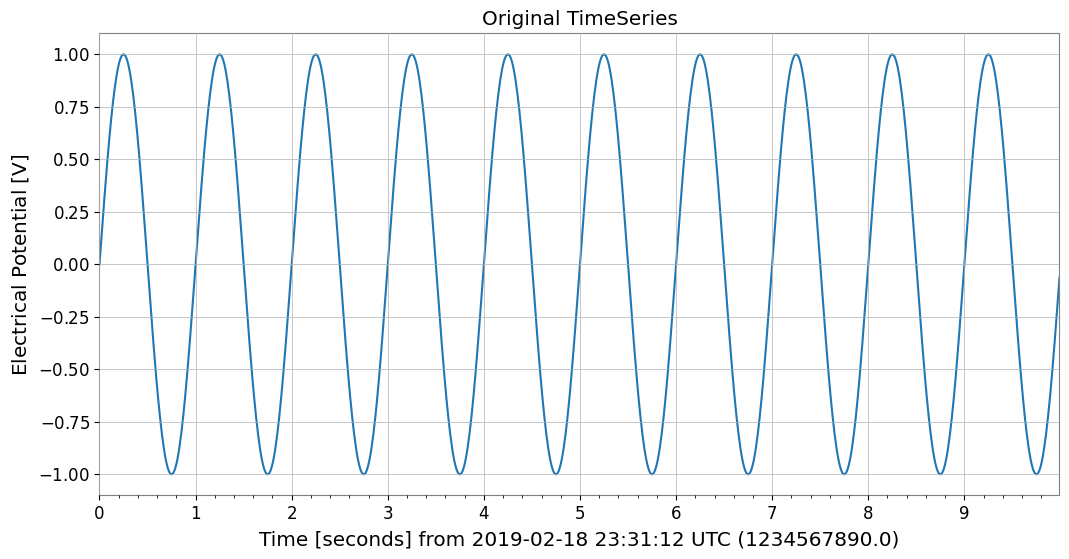
# Create sample data
# Generate a 10-second, 100Hz sine wave
rate = 100 * u.Hz
dt = 1 / rate
t0 = LIGOTimeGPS(1234567890, 0)
duration = 10 * u.s
size = int(rate * duration)
times = np.arange(size) * dt.value
data = np.sin(2 * np.pi * 1.0 * times)  # 1Hz sine wave

ts = TimeSeries(data, t0=t0, dt=dt, unit="V", name="demo_signal")
print("Original TimeSeries:")
print(ts)
ts.plot(title="Original TimeSeries");

Original TimeSeries:
TimeSeries([ 0.        ,  0.06279052,  0.12533323, ...,
            -0.18738131, -0.12533323, -0.06279052],
           unit: V,
           t0: 1234567890.0 1 / Hz,
           dt: 0.01 1 / Hz,
           name: demo_signal,
           channel: None)

1. General Data Formats & Data Infrastructure

1.1. NumPy [Original GWpy]

NumPy: NumPy is the foundational library for numerical computing in Python, providing multidimensional arrays and fast mathematical operations. 📚 NumPy Documentation

You can obtain NumPy arrays via TimeSeries.value or np.asarray(ts).

1.2. Pandas Integration [Original GWpy]

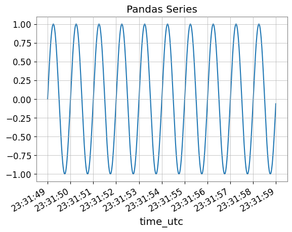
Pandas: Pandas is a powerful library for data analysis and manipulation, providing flexible data structures through DataFrame and Series. 📚 Pandas Documentation

Using the to_pandas() method, you can convert TimeSeries to pandas.Series. The index can be selected from datetime (UTC), gps, or seconds (Unix timestamp).

try:
    # Convert to Pandas Series (default is datetime index)
    s_pd = ts.to_pandas(index="datetime")
    print("\n--- Converted to Pandas Series ---")
    display(s_pd)
    s_pd.plot(title="Pandas Series")
    plt.show()
    plt.close()

    # Restore TimeSeries from Pandas Series
    ts_restored = TimeSeries.from_pandas(s_pd, unit="V")
    print("\n--- Restored TimeSeries from Pandas ---")
    print(ts_restored)

    del s_pd, ts_restored

except ImportError:
    print("Pandas is not installed.")

--- Converted to Pandas Series ---

time_utc
2019-02-18 23:31:49+00:00           0.000000
2019-02-18 23:31:49.010000+00:00    0.062791
2019-02-18 23:31:49.020000+00:00    0.125333
2019-02-18 23:31:49.030000+00:00    0.187381
2019-02-18 23:31:49.040000+00:00    0.248690
                                      ...
2019-02-18 23:31:58.949991+00:00   -0.309017
2019-02-18 23:31:58.959991+00:00   -0.248690
2019-02-18 23:31:58.969990+00:00   -0.187381
2019-02-18 23:31:58.979990+00:00   -0.125333
2019-02-18 23:31:58.989990+00:00   -0.062791
Name: demo_signal, Length: 1000, dtype: float64

--- Restored TimeSeries from Pandas ---
TimeSeries([ 0.        ,  0.06279052,  0.12533323, ...,
            -0.18738131, -0.12533323, -0.06279052],
           unit: V,
           t0: 1234567927.0 s,
           dt: 0.009999990463256836 s,
           name: demo_signal,
           channel: None)

1.3. Polars [GWExPy New]

Polars: Polars is a high-performance DataFrame library implemented in Rust, excelling at large-scale data processing. 📚 Polars Documentation

You can convert to Polars DataFrame/Series with to_polars().

try:
    import polars as pl

    _ = pl
    # TimeSeries -> Polars DataFrame
    df_pl = ts.to_polars()
    print("--- Polars DataFrame ---")
    print(df_pl.head())

    # Plot using Polars/Matplotlib
    plt.figure()
    data_col = [c for c in df_pl.columns if c != "time"][0]
    plt.plot(df_pl["time"], df_pl[data_col])
    plt.title("Polars Data Plot")
    plt.show()

    # Recover to TimeSeries
    from gwexpy.timeseries import TimeSeries

    ts_recovered = TimeSeries.from_polars(df_pl)
    print("Recovered from Polars:", ts_recovered)

    del df_pl, ts_recovered

except ImportError:
    print("Polars not installed.")

--- Polars DataFrame ---
shape: (5, 2)
┌────────────────────────────┬─────────────┐
│ time                       ┆ demo_signal │
│ ---                        ┆ ---         │
│ object                     ┆ f64         │
╞════════════════════════════╪═════════════╡
│ 2019-02-18 23:31:12        ┆ 0.0         │
│ 2019-02-18 23:31:12.010000 ┆ 0.062791    │
│ 2019-02-18 23:31:12.020000 ┆ 0.125333    │
│ 2019-02-18 23:31:12.030000 ┆ 0.187381    │
│ 2019-02-18 23:31:12.040000 ┆ 0.24869     │
└────────────────────────────┴─────────────┘

Recovered from Polars: TimeSeries([ 0.        ,  0.06279052,  0.12533323, ...,
            -0.18738131, -0.12533323, -0.06279052],
           unit: dimensionless,
           t0: 1234567890.0 s,
           dt: None,
           name: demo_signal,
           channel: None)

1.4. Xarray Integration [Original GWpy]

xarray: xarray is a library for multidimensional labeled arrays, widely used for manipulating NetCDF data and analyzing meteorological and earth science data. 📚 xarray Documentation

xarray is a powerful library for handling multidimensional labeled arrays. You can convert with to_xarray() while preserving metadata.

try:
    # Convert to Xarray DataArray
    da = ts.to_xarray()
    print("\n--- Converted to Xarray DataArray ---")
    print(da)
    # Verify metadata (attrs) is preserved
    print("Attributes:", da.attrs)

    da.plot()
    plt.title("Xarray DataArray")
    plt.show()
    plt.close()

    # Restore
    ts_x = TimeSeries.from_xarray(da)
    print("\n--- Restored TimeSeries from Xarray ---")
    print(ts_x)

    del da, ts_x

except ImportError:
    print("Xarray is not installed.")

--- Converted to Xarray DataArray ---
<xarray.DataArray 'demo_signal' (time: 1000)> Size: 8kB
array([ 0.        ,  0.06279052,  0.12533323, ..., -0.18738131,
       -0.12533323, -0.06279052], shape=(1000,))
Coordinates:
  * time     (time) datetime64[us] 8kB 2019-02-18T23:31:49 ... 2019-02-18T23:...
Attributes:
    unit:        V
    name:        demo_signal
    channel:     None
    epoch:       1234567890.0
    time_coord:  datetime
Attributes: {'unit': 'V', 'name': 'demo_signal', 'channel': 'None', 'epoch': 1234567890.0, 'time_coord': 'datetime'}

--- Restored TimeSeries from Xarray ---
TimeSeries([ 0.        ,  0.06279052,  0.12533323, ...,
            -0.18738131, -0.12533323, -0.06279052],
           unit: V,
           t0: 1234567927.0 s,
           dt: 0.009999990463256836 s,
           name: demo_signal,
           channel: None)

1.5. Dask Integration [GWExPy New]

Dask: Dask is a library for parallel computing that enables processing of large-scale data beyond NumPy/Pandas. 📚 Dask Documentation

try:
    import dask.array as da

    _ = da
    # Convert to Dask Array
    dask_arr = ts.to_dask(chunks="auto")
    print("\n--- Converted to Dask Array ---")
    print(dask_arr)

    # Restore (compute=True loads immediately)
    ts_from_dask = TimeSeries.from_dask(dask_arr, t0=ts.t0, dt=ts.dt, unit=ts.unit)
    print("Recovered from Dask:", ts_from_dask)

    del dask_arr, ts_from_dask

except ImportError:
    print("Dask not installed.")

--- Converted to Dask Array ---
dask.array<array, shape=(1000,), dtype=float64, chunksize=(1000,), chunktype=numpy.ndarray>
Recovered from Dask: TimeSeries([ 0.        ,  0.06279052,  0.12533323, ...,
            -0.18738131, -0.12533323, -0.06279052],
           unit: V,
           t0: 1234567890.0 1 / Hz,
           dt: 0.01 1 / Hz,
           name: None,
           channel: None)

1.6. JSON / Python Dict (to_json) [GWExPy New]

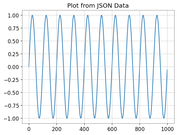
JSON: JSON (JavaScript Object Notation) is a lightweight data exchange format supported by the Python standard library. 📚 JSON Documentation

You can output JSON-compatible dictionary format with to_json() or to_dict().

import json

# TimeSeries -> JSON string
ts_json = ts.to_json()
print("--- JSON Representation (Partial) ---")
print(ts_json[:500] + "...")

# Plot data by loading back from JSON
ts_dict_temp = json.loads(ts_json)
plt.figure()
plt.plot(ts_dict_temp["data"])
plt.title("Plot from JSON Data")
plt.show()

# Recover from JSON
from gwexpy.timeseries import TimeSeries

ts_recovered = TimeSeries.from_json(ts_json)
print("Recovered from JSON:", ts_recovered)

del ts_json, ts_dict_temp, ts_recovered

--- JSON Representation (Partial) ---
{
  "t0": 1234567890.0,
  "dt": 0.01,
  "unit": "V",
  "name": "demo_signal",
  "data": [
    0.0,
    0.06279051952931337,
    0.12533323356430426,
    0.1873813145857246,
    0.2486898871648548,
    0.3090169943749474,
    0.3681245526846779,
    0.4257792915650727,
    0.4817536741017153,
    0.5358267949789967,
    0.5877852522924731,
    0.6374239897486896,
    0.6845471059286886,
    0.7289686274214116,
    0.7705132427757893,
    0.8090169943749475,
    0.8443279255020151,
    0.876306680...

Recovered from JSON: TimeSeries([ 0.        ,  0.06279052,  0.12533323, ...,
            -0.18738131, -0.12533323, -0.06279052],
           unit: V,
           t0: 1234567890.0 s,
           dt: 0.01 s,
           name: demo_signal,
           channel: None)

2. Database & Storage Layer

2.1. HDF5 [Original GWpy]

HDF5: HDF5 is a hierarchical data format for efficiently storing and managing large-scale scientific data. It can be accessed from Python via the h5py library. 📚 HDF5 Documentation

Supports saving to HDF5 with to_hdf5_dataset().

try:
    import tempfile

    import h5py

    with tempfile.NamedTemporaryFile(suffix=".h5") as tmp:
        # TimeSeries -> HDF5
        with h5py.File(tmp.name, "w") as f:
            ts.to_hdf5_dataset(f, "dataset_01")

        # Read back and display
        with h5py.File(tmp.name, "r") as f:
            ds = f["dataset_01"]
            print("--- HDF5 Dataset Info ---")
            print(f"Shape: {ds.shape}, Dtype: {ds.dtype}")
            print("Attributes:", dict(ds.attrs))

            # Recover
            from gwexpy.timeseries import TimeSeries

            ts_recovered = TimeSeries.from_hdf5_dataset(f, "dataset_01")
            print("Recovered from HDF5:", ts_recovered)

            ts_recovered.plot()
            plt.title("Recovered from HDF5")
            plt.show()

            del ds, ts_recovered

except ImportError:
    print("h5py not installed.")

--- HDF5 Dataset Info ---
Shape: (1000,), Dtype: float64
Attributes: {'dt': np.float64(0.01), 'name': 'demo_signal', 't0': np.float64(1234567890.0), 'unit': 'V'}
Recovered from HDF5: TimeSeries([ 0.        ,  0.06279052,  0.12533323, ...,
            -0.18738131, -0.12533323, -0.06279052],
           unit: V,
           t0: 1234567890.0 s,
           dt: 0.01 s,
           name: demo_signal,
           channel: None)

2.2. SQLite [GWExPy New]

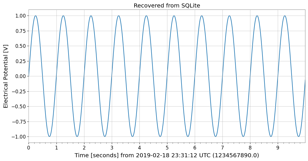
SQLite: SQLite is a lightweight embedded SQL database engine included in the Python standard library. 📚 SQLite Documentation

Supports database persistence with to_sqlite().

import sqlite3

conn = sqlite3.connect(":memory:")

# TimeSeries -> SQLite
series_id = ts.to_sqlite(conn, series_id="test_series")
print(f"Saved to SQLite with ID: {series_id}")

# Verify data in SQL
cursor = conn.cursor()
row = cursor.execute("SELECT * FROM series WHERE series_id=?", (series_id,)).fetchone()
print("Metadata from SQL:", row)

# Recover
from gwexpy.timeseries import TimeSeries

ts_recovered = TimeSeries.from_sqlite(conn, series_id)
print("Recovered from SQLite:", ts_recovered)

ts_recovered.plot()
plt.title("Recovered from SQLite")
plt.show()

del series_id, conn, cursor, ts_recovered

Saved to SQLite with ID: test_series
Metadata from SQL: ('test_series', '', 'V', 1234567890.0, 0.01, 1000, '{"name": "demo_signal"}')
Recovered from SQLite: TimeSeries([ 0.        ,  0.06279052,  0.12533323, ...,
            -0.18738131, -0.12533323, -0.06279052],
           unit: V,
           t0: 1234567890.0 s,
           dt: 0.01 s,
           name: test_series,
           channel: None)

2.3. Zarr [GWExPy New]

Zarr: Zarr is a storage format for chunked, compressed multidimensional arrays with excellent cloud storage integration. 📚 Zarr Documentation

Supports cloud storage-friendly formats with to_zarr().

try:
    import os
    import tempfile

    import zarr

    with tempfile.TemporaryDirectory() as tmpdir:
        store_path = os.path.join(tmpdir, "test.zarr")
        # TimeSeries -> Zarr
        ts.to_zarr(store_path, path="timeseries")

        # Read back
        z = zarr.open(store_path, mode="r")
        ds = z["timeseries"]
        print("--- Zarr Array Info ---")
        print(ds.info)

        # Recover
        from gwexpy.timeseries import TimeSeries

        ts_recovered = TimeSeries.from_zarr(store_path, "timeseries")
        print("Recovered from Zarr:", ts_recovered)

        ts_recovered.plot()
        plt.title("Recovered from Zarr")
        plt.show()

        del z, ds, ts_recovered

except ImportError:
    print("zarr not installed.")

--- Zarr Array Info ---
Type               : Array
Zarr format        : 3
Data type          : Float64(endianness='little')
Fill value         : 0.0
Shape              : (1000,)
Chunk shape        : (1000,)
Order              : C
Read-only          : True
Store type         : LocalStore
Filters            : ()
Serializer         : BytesCodec(endian=<Endian.little: 'little'>)
Compressors        : (ZstdCodec(level=0, checksum=False),)
No. bytes          : 8000 (7.8K)
Recovered from Zarr: TimeSeries([ 0.        ,  0.06279052,  0.12533323, ...,
            -0.18738131, -0.12533323, -0.06279052],
           unit: V,
           t0: 1234567890.0 s,
           dt: 0.01 s,
           name: demo_signal,
           channel: None)

2.4. netCDF4 [GWExPy New]

netCDF4: netCDF4 is a standard format for meteorological, oceanographic, and earth science data with self-describing data structures. 📚 netCDF4 Documentation

Supports meteorological and oceanographic data standards with to_netcdf4().

try:
    import tempfile
    from pathlib import Path

    import netCDF4

    with tempfile.TemporaryDirectory() as tmpdir:
        path = Path(tmpdir) / "gwexpy_timeseries.nc"

        # TimeSeries -> netCDF4
        with netCDF4.Dataset(path, "w", format="NETCDF3_CLASSIC") as ds:
            ts.to_netcdf4(ds, "my_signal")

        # Read back
        with netCDF4.Dataset(path, "r") as ds:
            v = ds.variables["my_signal"]
            print("--- netCDF4 Variable Info ---")
            print(v)

            # Recover
            from gwexpy.timeseries import TimeSeries

            ts_recovered = TimeSeries.from_netcdf4(ds, "my_signal")
            print("Recovered from netCDF4:", ts_recovered)

            ts_recovered.plot()
            plt.title("Recovered from netCDF4")
            plt.show()

            del v, ts_recovered

except ImportError:
    print("netCDF4 not installed.")

--- netCDF4 Variable Info ---
<class 'netCDF4.Variable'>
float64 my_signal(time)
    t0: 1234567890.0
    dt: 0.01
    units: V
    long_name: demo_signal
unlimited dimensions:
current shape = (1000,)
filling on, default _FillValue of 9.969209968386869e+36 used
Recovered from netCDF4: TimeSeries([ 0.        ,  0.06279052,  0.12533323, ...,
            -0.18738131, -0.12533323, -0.06279052],
           unit: V,
           t0: 1234567890.0 s,
           dt: 0.01 s,
           name: demo_signal,
           channel: None)

3. Computer Science, Machine Learning & Accelerated Computing

3.1. PyTorch Integration [GWExPy New]

PyTorch: PyTorch is a deep learning framework supporting dynamic computation graphs and GPU acceleration. 📚 PyTorch Documentation

For deep learning preprocessing, you can directly convert TimeSeries to torch.Tensor. GPU transfer is also supported.

import os

os.environ.setdefault("TF_CPP_MIN_LOG_LEVEL", "3")

try:
    import torch

    # Convert to PyTorch Tensor
    tensor = ts.to_torch(dtype=torch.float32)
    print("\n--- Converted to PyTorch Tensor ---")
    print(f"Tensor shape: {tensor.shape}, dtype: {tensor.dtype}")

    # Restore from Tensor (t0, dt must be specified separately)
    ts_torch = TimeSeries.from_torch(tensor, t0=ts.t0, dt=ts.dt, unit="V")
    print("\n--- Restored from Torch ---")
    print(ts_torch)

    del tensor, ts_torch

except ImportError:
    print("PyTorch is not installed.")

--- Converted to PyTorch Tensor ---
Tensor shape: torch.Size([1000]), dtype: torch.float32

--- Restored from Torch ---
TimeSeries([ 0.        ,  0.06279052,  0.12533323, ...,
            -0.18738131, -0.12533323, -0.06279052],
           unit: V,
           t0: 1234567890.0 1 / Hz,
           dt: 0.01 1 / Hz,
           name: None,
           channel: None)

3.2. CuPy (CUDA Acceleration) [GWExPy New]

CuPy: CuPy is a NumPy-compatible GPU array library that enables high-speed computation using NVIDIA CUDA. 📚 CuPy Documentation

You can convert to CuPy arrays for GPU-based computation.

from gwexpy.interop import is_cupy_available

if is_cupy_available():
    import cupy as cp

    # TimeSeries -> CuPy
    y_gpu = ts.to_cupy()
    print("--- CuPy Array (on GPU) ---")
    print(y_gpu)

    # Simple processing on GPU
    y_gpu_filt = y_gpu * 2.0

    # Plot (must move to CPU for plotting)
    plt.figure()
    plt.plot(cp.asnumpy(y_gpu_filt))
    plt.title("CuPy Data (Moved to CPU for plot)")
    plt.show()

    # Recover
    from gwexpy.timeseries import TimeSeries

    ts_recovered = TimeSeries.from_cupy(y_gpu_filt, t0=ts.t0, dt=ts.dt)
    print("Recovered from CuPy:", ts_recovered)

    del y_gpu, y_gpu_filt, ts_recovered

else:
    print("CuPy or CUDA driver not available.")

CuPy or CUDA driver not available.

3.3. TensorFlow Integration [GWExPy New]

TensorFlow: TensorFlow is a machine learning platform developed by Google, excelling at large-scale production environments. 📚 TensorFlow Documentation

try:
    import os
    import warnings

    os.environ.setdefault("TF_CPP_MIN_LOG_LEVEL", "3")
    warnings.filterwarnings(
        "ignore", category=UserWarning, module=r"google\.protobuf\..*"
    )
    warnings.filterwarnings(
        "ignore", category=UserWarning, message=r"Protobuf gencode version.*"
    )
    import tensorflow as tf

    _ = tf
    # Convert to TensorFlow Tensor
    tf_tensor = ts.to_tensorflow()
    print("\n--- Converted to TensorFlow Tensor ---")
    print(f"Tensor shape: {tf_tensor.shape}")
    print(f"Tensor dtype: {tf_tensor.dtype}")

    # Restore
    ts_from_tensorflow = TimeSeries.from_tensorflow(
        tf_tensor, t0=ts.t0, dt=ts.dt, unit=ts.unit
    )
    print("Recovered from TF:", ts_from_tensorflow)

    del tf_tensor, ts_from_tensorflow

except ImportError:
    pass

3.4. JAX Integration [GWExPy New]

JAX: JAX is a high-performance numerical computing library developed by Google, featuring automatic differentiation and XLA compilation for acceleration. 📚 JAX Documentation

try:
    import os

    os.environ["XLA_PYTHON_CLIENT_PREALLOCATE"] = "false"
    import jax

    _ = jax
    import jax.numpy as jnp

    _ = jnp
    # Convert to JAX Array
    jax_arr = ts.to_jax()
    print("\n--- Converted to JAX Array ---")
    print(f"Array shape: {jax_arr.shape}")

    # Restore
    ts_from_jax = TimeSeries.from_jax(jax_arr, t0=ts.t0, dt=ts.dt, unit=ts.unit)
    print("Recovered from JAX:", ts_from_jax)

    del jax_arr, ts_from_jax
except ImportError:
    print("JAX not installed.")

--- Converted to JAX Array ---
Array shape: (1000,)
Recovered from JAX: TimeSeries([ 0.        ,  0.06279052,  0.12533323, ...,
            -0.18738131, -0.12533323, -0.06279052],
           unit: V,
           t0: 1234567890.0 1 / Hz,
           dt: 0.01 1 / Hz,
           name: None,
           channel: None)

4. Astronomy & Gravitational Wave Physics

4.1. PyCBC / LAL [Original GWpy]

LAL: LAL (LIGO Algorithm Library) is the official analysis library for LIGO/Virgo, providing the foundation for gravitational wave analysis. 📚 LAL Documentation

PyCBC: PyCBC is a library for gravitational wave data analysis, used for signal searches and parameter estimation. 📚 PyCBC Documentation

Provides compatibility with standard gravitational wave analysis tools.

4.2. Astropy Integration [Original GWpy]

Astropy: Astropy is a Python library for astronomy, supporting coordinate transformations, time system conversions, unit systems, and more. 📚 Astropy Documentation

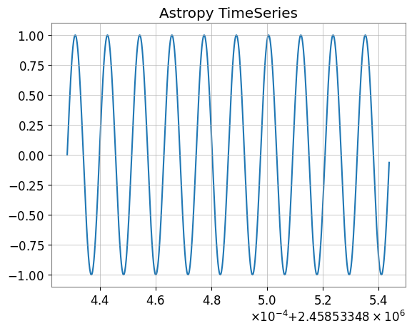
Also supports interconversion with astropy.timeseries.TimeSeries, which is standard in the astronomy field.

try:
    # Convert to Astropy TimeSeries
    ap_ts = ts.to_astropy_timeseries()
    print("\n--- Converted to Astropy TimeSeries ---")
    print(ap_ts[:5])
    fig, ax = plt.subplots()
    ax.plot(ap_ts.time.jd, ap_ts["value"])
    plt.title("Astropy TimeSeries")
    plt.show()
    plt.close()

    # Restore
    ts_astro = TimeSeries.from_astropy_timeseries(ap_ts)
    print("\n--- Restored from Astropy ---")
    print(ts_astro)

    del ap_ts, ts_astro

except ImportError:
    print("Astropy is not installed.")

--- Converted to Astropy TimeSeries ---
     time            value
------------- -------------------
 1234567890.0                 0.0
1234567890.01 0.06279051952931337
1234567890.02 0.12533323356430426
1234567890.03  0.1873813145857246
1234567890.04  0.2486898871648548

--- Restored from Astropy ---
TimeSeries([ 0.        ,  0.06279052,  0.12533323, ...,
            -0.18738131, -0.12533323, -0.06279052],
           unit: dimensionless,
           t0: 1234567890.0 s,
           dt: 0.009999990463256836 s,
           name: None,
           channel: None)

4.3. Specutils Integration [GWExPy New]

specutils: specutils is an Astropy-affiliated package for manipulating and analyzing astronomical spectral data. 📚 specutils Documentation

FrequencySeries can interconvert with Spectrum1D objects from the Astropy ecosystem spectral analysis library specutils. Units and frequency axes are properly preserved.

try:
    import specutils

    _ = specutils

    from gwexpy.frequencyseries import FrequencySeries

    # FrequencySeries -> specutils.Spectrum1D
    fs = FrequencySeries(
        np.random.random(100), frequencies=np.linspace(10, 100, 100), unit="Jy"
    )
    spec = fs.to_specutils()
    print("specutils Spectrum1D:", spec)
    print("Spectral axis unit:", spec.spectral_axis.unit)

    # specutils.Spectrum1D -> FrequencySeries
    fs_rec = FrequencySeries.from_specutils(spec)
    print("Restored FrequencySeries unit:", fs_rec.unit)

    del fs, spec, fs_rec

except ImportError:
    print("specutils library not found. Skipping example.")

specutils Spectrum1D: Spectrum (length=100)
Flux=[0.4996616  0.87200803 0.91825306 ... 0.90868047 0.91147843
      0.98486678] Jy,  mean=0.49949 Jy
Spectral Axis=[ 10.          10.90909091  11.81818182 ...
                98.18181818  99.09090909 100.        ] Hz,  mean=55.00000 Hz
Spectral axis unit: Hz
Restored FrequencySeries unit: Jy

4.4. Pyspeckit Integration [GWExPy New]

PySpecKit: PySpecKit is a spectral analysis toolkit for radio astronomy, supporting spectral line fitting and more. 📚 PySpecKit Documentation

FrequencySeries can also integrate with Spectrum objects from the general-purpose spectral analysis toolkit pyspeckit.

try:
    import pyspeckit

    _ = pyspeckit
    from gwexpy.frequencyseries import FrequencySeries

    # FrequencySeries -> pyspeckit.Spectrum
    fs = FrequencySeries(np.random.random(100), frequencies=np.linspace(10, 100, 100))
    spec = fs.to_pyspeckit()
    print("pyspeckit Spectrum length:", len(spec.data))

    # pyspeckit.Spectrum -> FrequencySeries
    fs_rec = FrequencySeries.from_pyspeckit(spec)
    print("Restored FrequencySeries length:", len(fs_rec))

    del fs, spec, fs_rec

except ImportError:
    print("pyspeckit library not found. Skipping example.")

pyspeckit Spectrum length: 100
Restored FrequencySeries length: 100

WARNING: No header given.  Creating an empty one.

5. Particle Physics & High Energy Physics

5.1. CERN ROOT Integration [GWExPy New]

ROOT: ROOT is a data analysis framework for high-energy physics developed by CERN. 📚 ROOT Documentation

Enhanced interoperability with ROOT, the standard tool in high-energy physics. gwexpy Series objects can be quickly converted to ROOT’s TGraph, TH1D, or TH2D, and you can create ROOT files. Conversely, you can also restore TimeSeries and other objects from ROOT objects.

Note: Using this feature requires ROOT (PyROOT) to be installed.

try:
    import numpy as np
    import ROOT

    from gwexpy.timeseries import TimeSeries

    # Prepare data
    t = np.linspace(0, 10, 1000)
    data = np.sin(2 * np.pi * 1.0 * t) + np.random.normal(0, 0.5, size=len(t))
    ts = TimeSeries(data, dt=t[1] - t[0], name="signal")

    # --- 1. Convert to TGraph ---
    # Vectorized high-speed conversion
    graph = ts.to_tgraph()

    # Plot on ROOT canvas
    c1 = ROOT.TCanvas("c1", "TGraph Example", 800, 600)
    graph.SetTitle("ROOT TGraph;GPS Time [s];Amplitude")
    graph.Draw("AL")
    c1.Draw()
    # c1.SaveAs("signal_graph.png") # To save as an image

    print(f"Created TGraph: {graph.GetName()} with {graph.GetN()} points")

    # --- 2. Convert to TH1D (Histogram) ---
    # Convert as histogram (binning is automatic or can be specified)
    hist = ts.to_th1d()

    c2 = ROOT.TCanvas("c2", "TH1D Example", 800, 600)
    hist.SetTitle("ROOT TH1D;GPS Time [s];Amplitude")
    hist.SetLineColor(ROOT.kRed)
    hist.Draw()
    c2.Draw()

    print(f"Created TH1D: {hist.GetName()} with {hist.GetNbinsX()} bins")

    del t, data, graph, hist, c1, c2

except ImportError:
    pass
except Exception as e:
    print(f"An error occurred: {e}")

5.2. Recovering from ROOT Objects (from_root)

ROOT: ROOT is a data analysis framework for high-energy physics developed by CERN. 📚 ROOT Documentation

You can load histograms and graphs from existing ROOT files and convert them back to gwexpy objects for easier analysis.

try:
    if "hist" in locals() and hist:
        # ROOT TH1D -> TimeSeries
        # Reads histogram bin contents as time series data
        ts_restored = from_root(TimeSeries, hist)

        print(f"Restored TimeSeries: {ts_restored.name}")
        print(ts_restored)

        # Restore from TGraph similarly
        ts_from_graph = from_root(TimeSeries, graph)
        print(f"Restored from TGraph: {len(ts_from_graph)} samples")

        del ts_restored, ts_from_graph

except NameError:
    pass  # If hist or graph were not created
except ImportError:
    pass

6. Geophysics, Seismology & Electromagnetics

6.1. ObsPy [Original GWpy]

ObsPy: ObsPy is a Python library for acquiring, processing, and analyzing seismological data, supporting formats like MiniSEED. 📚 ObsPy Documentation

Supports interoperability with ObsPy, which is standard in seismology.

try:
    import obspy

    _ = obspy
    # TimeSeries -> ObsPy Trace
    tr = ts.to_obspy()
    print("--- ObsPy Trace ---")
    print(tr)

    # Plot using ObsPy
    tr.plot()

    # Recover to TimeSeries
    from gwexpy.timeseries import TimeSeries

    ts_recovered = TimeSeries.from_obspy(tr)
    print("Recovered from ObsPy:", ts_recovered)

    del tr, ts_recovered

except ImportError:
    print("ObsPy not installed.")

--- ObsPy Trace ---
.demo_signal.. | 2019-02-18T23:31:12.000000Z - 2019-02-18T23:31:21.990000Z | 100.0 Hz, 1000 samples

Recovered from ObsPy: TimeSeries([ 0.        ,  0.06279052,  0.12533323, ...,
            -0.18738131, -0.12533323, -0.06279052],
           unit: dimensionless,
           t0: 1234567890.0 s,
           dt: 0.01 s,
           name: .demo_signal..,
           channel: None)

try:
    import obspy

    _ = obspy
    tr = ts.to_obspy()
    print("ObsPy Trace:", tr)

    del tr

except ImportError:
    print("ObsPy not installed.")

ObsPy Trace: .demo_signal.. | 2019-02-18T23:31:12.000000Z - 2019-02-18T23:31:21.990000Z | 100.0 Hz, 1000 samples

6.2. SimPEG Integration [GWExPy New]

SimPEG: SimPEG is a simulation and estimation framework for geophysical inverse problems. 📚 SimPEG Documentation

gwexpy supports integration with SimPEG, a forward modeling and inversion library for geophysics. TimeSeries (TDEM) and FrequencySeries (FDEM) can be converted to simpeg.data.Data objects and vice versa.

try:
    import numpy as np
    import simpeg

    _ = simpeg
    from simpeg import maps

    _ = maps

    from gwexpy.frequencyseries import FrequencySeries
    from gwexpy.timeseries import TimeSeries

    # --- TimeSeries -> SimPEG (TDEM assumption) ---
    ts = TimeSeries(np.random.normal(size=100), dt=0.01, unit="A/m^2")
    simpeg_data_td = ts.to_simpeg(location=np.array([0, 0, 0]))
    print("SimPEG TDEM data shape:", simpeg_data_td.dobs.shape)

    # --- FrequencySeries -> SimPEG (FDEM assumption) ---
    fs = FrequencySeries(
        np.random.normal(size=10) + 1j * 0.1, frequencies=np.logspace(0, 3, 10)
    )
    simpeg_data_fd = fs.to_simpeg(location=np.array([0, 0, 0]), orientation="z")
    print("SimPEG FDEM data shape:", simpeg_data_fd.dobs.shape)

    del simpeg_data_td, simpeg_data_fd, fs

except ImportError:
    print("SimPEG library not found. Skipping example.")

SimPEG TDEM data shape: (100,)
SimPEG FDEM data shape: (10,)

6.3. MTH5 / MTpy [GWExPy New]

MTH5: MTH5 is an HDF5-based data format for magnetotelluric (MT) data. 📚 MTH5 Documentation

Supports MTH5 storage for magnetotelluric method data.

try:
    import logging
    import tempfile

    logging.getLogger("mth5").setLevel(logging.ERROR)
    logging.getLogger("mt_metadata").setLevel(logging.ERROR)

    import mth5

    _ = mth5
    with tempfile.NamedTemporaryFile(suffix=".h5") as tmp:
        from gwexpy.interop.mt_ import from_mth5, to_mth5

        # TimeSeries -> MTH5
        # We need to provide station and run names for MTH5 structure
        to_mth5(ts, tmp.name, station="SITE01", run="RUN01")
        print(f"Saved to MTH5 file: {tmp.name}")

        # Display structure info if needed, or just recover
        # Recover
        ts_recovered = from_mth5(tmp.name, "SITE01", "RUN01", ts.name or "Ex")
        print("Recovered from MTH5:", ts_recovered)

        ts_recovered.plot()
        plt.title("Recovered from MTH5")
        plt.show()

        del ts_recovered

except ImportError:
    print("mth5 not installed.")

2026-02-26T20:43:07.864620+0900 | INFO | mth5.mth5 | _initialize_file | line: 900 | Initialized MTH5 0.2.0 file /tmp/tmp99d3d2q2.h5 in mode a
2026-02-26T20:43:08.559892+0900 | INFO | mth5.mth5 | close_mth5 | line: 1035 | Flushing and closing /tmp/tmp99d3d2q2.h5
Saved to MTH5 file: /tmp/tmp99d3d2q2.h5
2026-02-26T20:43:08.809406+0900 | INFO | mth5.mth5 | close_mth5 | line: 1035 | Flushing and closing /tmp/tmp99d3d2q2.h5
Recovered from MTH5: TimeSeries([-1.27391684, -0.30269384, -2.00603464,  0.05845388,
             1.0126355 ,  0.33787515,  0.75505316,  0.05358523,
             0.38864351, -1.44961328,  1.08042893, -1.70999975,
             1.28250087,  1.55483424, -1.53453063,  0.74587519,
             1.15601664,  0.79389252, -0.97256545, -1.00021471,
             0.77242056,  0.94591899, -0.54435776,  0.77953267,
            -2.22549221,  0.65677856, -0.41458701,  0.66564574,
            -0.4295487 ,  0.87899976,  1.21903806, -0.22710473,
             0.32353946,  0.0360012 ,  1.55640423,  1.37184076,
            -0.90355895, -0.94101394,  0.12791804, -0.07807064,
            -0.48663129, -1.39614401,  1.69575536, -0.35566849,
             0.23237241,  0.44114807, -1.61365759, -0.01337514,
             0.87644533,  1.06702784,  1.87474203, -0.78545807,
             1.9774588 ,  1.37413999,  1.62586739,  0.61497643,
             1.2093394 , -0.14839093, -0.23969175,  0.21439602,
             0.12955564, -1.87875851, -1.51030825,  0.07133941,
            -0.91967009, -0.58081854, -1.10387025, -1.75364443,
            -0.2118928 , -0.28202094, -0.1271344 , -1.37538233,
            -0.45239899, -0.07999768,  2.41681807,  0.18291115,
            -1.9771057 , -0.07484536,  1.83648103, -0.68403258,
            -0.22077894, -0.38216236, -0.5267697 ,  0.53938925,
            -1.00988604, -1.15615062,  1.25724486,  0.23340044,
            -0.66255157,  1.30172765,  0.74012156,  0.15562436,
             1.12611035,  0.99886303, -0.21220112, -0.48088469,
             0.07853538,  1.18181081,  0.45684885, -1.01421591],
           unit: dimensionless,
           t0: 0.0 s,
           dt: 1.0 s,
           name: Ex,
           channel: None)

7. Acoustics & Audio Analysis

7.1. Librosa / Pydub [GWExPy New]

pydub: pydub is a simple library for audio file manipulation (editing, conversion, effects). 📚 pydub Documentation

librosa: librosa is a library for audio and music analysis, providing features like spectral analysis and beat detection. 📚 librosa Documentation

Supports integration with audio processing libraries Librosa and Pydub.

try:
    import librosa

    _ = librosa
    import matplotlib.pyplot as plt

    # TimeSeries -> Librosa (y, sr)
    y, sr = ts.to_librosa()
    print(f"--- Librosa Data ---\nSignal shape: {y.shape}, Sample rate: {sr}")

    # Plot using librosa style (matplotlib)
    plt.figure()
    plt.plot(y[:1000])  # Plot first 1000 samples
    plt.title("Librosa Audio Signal (Zoom)")
    plt.show()

    # Recover to TimeSeries
    from gwexpy.timeseries import TimeSeries

    ts_recovered = TimeSeries(y, dt=1.0 / sr)
    print("Recovered from Librosa:", ts_recovered)

    del y, sr
except ImportError:
    print("Librosa not installed.")

--- Librosa Data ---
Signal shape: (100,), Sample rate: 100

Recovered from Librosa: TimeSeries([-1.2739168 , -0.30269384, -2.0060346 ,  0.05845388,
             1.0126355 ,  0.33787516,  0.75505316,  0.05358523,
             0.3886435 , -1.4496133 ,  1.080429  , -1.7099998 ,
             1.2825009 ,  1.5548342 , -1.5345306 ,  0.7458752 ,
             1.1560166 ,  0.7938925 , -0.9725655 , -1.0002147 ,
             0.7724206 ,  0.945919  , -0.5443578 ,  0.7795327 ,
            -2.2254922 ,  0.6567786 , -0.41458702,  0.6656457 ,
            -0.4295487 ,  0.87899977,  1.219038  , -0.22710474,
             0.32353947,  0.0360012 ,  1.5564042 ,  1.3718407 ,
            -0.90355897, -0.94101393,  0.12791803, -0.07807064,
            -0.4866313 , -1.396144  ,  1.6957554 , -0.3556685 ,
             0.23237242,  0.44114807, -1.6136576 , -0.01337514,
             0.87644535,  1.0670278 ,  1.874742  , -0.7854581 ,
             1.9774588 ,  1.37414   ,  1.6258674 ,  0.6149764 ,
             1.2093394 , -0.14839093, -0.23969175,  0.21439601,
             0.12955564, -1.8787585 , -1.5103083 ,  0.07133941,
            -0.9196701 , -0.58081853, -1.1038703 , -1.7536445 ,
            -0.2118928 , -0.28202096, -0.1271344 , -1.3753823 ,
            -0.452399  , -0.07999767,  2.4168181 ,  0.18291114,
            -1.9771057 , -0.07484536,  1.836481  , -0.68403256,
            -0.22077894, -0.38216236, -0.5267697 ,  0.53938925,
            -1.009886  , -1.1561506 ,  1.2572448 ,  0.23340045,
            -0.6625516 ,  1.3017277 ,  0.74012154,  0.15562436,
             1.1261103 ,  0.99886304, -0.21220112, -0.4808847 ,
             0.07853539,  1.1818109 ,  0.45684886, -1.014216  ],
           unit: dimensionless,
           t0: 0.0 s,
           dt: 0.01 s,
           name: None,
           channel: None)

8. Medical & Biosignal Analysis

8.1. MNE-Python [GWExPy New]

MNE: MNE-Python is a library for analyzing EEG and MEG data, widely used in neuroscience research. 📚 MNE Documentation

Integration with MNE for electroencephalography (EEG/MEG) analysis packages.

try:
    import mne

    _ = mne
    # TimeSeries -> MNE Raw
    raw = ts.to_mne()
    print("--- MNE Raw ---")
    print(raw)

    # Display info
    print(raw.info)

    # Recover to TimeSeries
    from gwexpy.timeseries import TimeSeries

    ts_recovered = TimeSeries.from_mne(raw, channel=ts.name or "ch0")
    print("Recovered from MNE:", ts_recovered)

    del raw, ts_recovered

except ImportError:
    print("MNE not installed.")

Creating RawArray with float64 data, n_channels=1, n_times=100
    Range : 0 ... 99 =      0.000 ...     0.990 secs
Ready.
--- MNE Raw ---
<RawArray | 1 x 100 (1.0 s), ~6 KiB, data loaded>
<Info | 7 non-empty values
 bads: []
 ch_names: ch0
 chs: 1 misc
 custom_ref_applied: False
 highpass: 0.0 Hz
 lowpass: 50.0 Hz
 meas_date: unspecified
 nchan: 1
 projs: []
 sfreq: 100.0 Hz
>
Recovered from MNE: TimeSeries([-1.27391684, -0.30269384, -2.00603464,  0.05845388,
             1.0126355 ,  0.33787515,  0.75505316,  0.05358523,
             0.38864351, -1.44961328,  1.08042893, -1.70999975,
             1.28250087,  1.55483424, -1.53453063,  0.74587519,
             1.15601664,  0.79389252, -0.97256545, -1.00021471,
             0.77242056,  0.94591899, -0.54435776,  0.77953267,
            -2.22549221,  0.65677856, -0.41458701,  0.66564574,
            -0.4295487 ,  0.87899976,  1.21903806, -0.22710473,
             0.32353946,  0.0360012 ,  1.55640423,  1.37184076,
            -0.90355895, -0.94101394,  0.12791804, -0.07807064,
            -0.48663129, -1.39614401,  1.69575536, -0.35566849,
             0.23237241,  0.44114807, -1.61365759, -0.01337514,
             0.87644533,  1.06702784,  1.87474203, -0.78545807,
             1.9774588 ,  1.37413999,  1.62586739,  0.61497643,
             1.2093394 , -0.14839093, -0.23969175,  0.21439602,
             0.12955564, -1.87875851, -1.51030825,  0.07133941,
            -0.91967009, -0.58081854, -1.10387025, -1.75364443,
            -0.2118928 , -0.28202094, -0.1271344 , -1.37538233,
            -0.45239899, -0.07999768,  2.41681807,  0.18291115,
            -1.9771057 , -0.07484536,  1.83648103, -0.68403258,
            -0.22077894, -0.38216236, -0.5267697 ,  0.53938925,
            -1.00988604, -1.15615062,  1.25724486,  0.23340044,
            -0.66255157,  1.30172765,  0.74012156,  0.15562436,
             1.12611035,  0.99886303, -0.21220112, -0.48088469,
             0.07853538,  1.18181081,  0.45684885, -1.01421591],
           unit: dimensionless,
           t0: 0.0 s,
           dt: 0.01 s,
           name: ch0,
           channel: None)

try:
    import mne

    _ = mne
    raw = ts.to_mne()
    print("MNE Raw:", raw)

    del raw
except ImportError:
    print("MNE not installed.")

Creating RawArray with float64 data, n_channels=1, n_times=100
    Range : 0 ... 99 =      0.000 ...     0.990 secs
Ready.
MNE Raw: <RawArray | 1 x 100 (1.0 s), ~6 KiB, data loaded>

8.2. Elephant / quantities Integration [GWExPy New]

gwexpy’s FrequencySeries and Spectrogram can interconvert with quantities.Quantity objects. This is useful for integration with Elephant and Neo.

Note: Requires pip install quantities beforehand.

try:
    import numpy as np
    import quantities as pq

    _ = pq
    from gwexpy.frequencyseries import FrequencySeries

    # Create FrequencySeries
    freqs = np.linspace(0, 100, 101)
    data_fs = np.random.random(101)
    fs = FrequencySeries(data_fs, frequencies=freqs, unit="V")

    # to_quantities
    q_obj = fs.to_quantities(units="mV")
    print("Quantities object:", q_obj)

    # from_quantities
    fs_new = FrequencySeries.from_quantities(q_obj, frequencies=freqs)
    print("Restored FrequencySeries unit:", fs_new.unit)

    del freqs, data_fs, fs, q_obj, fs_new

except ImportError:
    print("quantities library not found. Skipping example.")

Quantities object: [841.93305592 518.04016791 452.69429198 563.24344871
 973.77492479 698.11123948 149.5312924  565.12006233
 364.50256071 129.92049363 710.75208837  63.17884694
 785.34147378 136.77526946 123.29383213 506.14709256
 162.94820574 642.79250323 471.94196377 645.04609794
 267.57854177 147.19549679 781.91812778 868.50806828
 668.12562908 566.04132528 281.75412162 101.84056854
 180.73610389 218.3133094  703.02667783  86.79431693
 786.04173329 215.05550329 935.61263196  82.10358717
 659.70668052 739.33495665  82.8131954  496.09033211
 509.67134141 483.54276605 669.68921827 342.2568704
 764.81961673 712.87057454 851.76682158 390.29533834
 831.87199183 584.43010877 178.62279577 732.91645393
 178.5035719   23.38133531 778.89361647 144.57882829
 134.14036961 424.98528463 845.2221757  519.39456465
 918.58055997 252.82560428 144.27322088 767.34008145
 716.83018817 540.80387596 839.33829692 269.66128911
 448.09240226 312.80135145 693.08971949 443.25157103
 537.7096665  254.31337586 275.6370865  673.4391078
 814.88480911 466.93143242  33.86723136 612.24975264
  15.83023827 288.21640646 848.90153772 543.70050635
 872.72135973 898.76545561 274.59135565 116.41752459
 686.91859471 949.52206081  54.57019727 726.52076052
 425.12213615  78.95659607 254.07135461 474.40040205
 523.35301986 941.66865426 404.10472364 132.68149548
 834.86049899] mV
Restored FrequencySeries unit: mV

8.3. Neo [GWExPy New]

Neo: Neo is a data structure library for electrophysiology data (neuroscience), supporting input/output to various formats. 📚 Neo Documentation

Supports conversion to Neo, a common standard for electrophysiological data.

try:
    import neo

    _ = neo
    # TimeSeries -> Neo AnalogSignal
    # to_neo is available in gwexpy.interop
    # Note: TimeseriesMatrix is preferred for multi-channel Neo conversion,
    # but we can convert single TimeSeries by wrapping it.
    from gwexpy.interop import from_neo, to_neo

    _ = from_neo
    _ = to_neo
    # For single TimeSeries, we might need a Matrix wrapper or direct helper.
    # Assuming helper exists or using Matrix:
    from gwexpy.timeseries import TimeSeriesMatrix

    tm = TimeSeriesMatrix(
        ts.value[None, None, :], t0=ts.t0, dt=ts.dt, channel_names=[ts.name]
    )
    sig = tm.to_neo()

    print("--- Neo AnalogSignal ---")
    print(sig)

    # Display/Plot
    plt.figure()
    plt.plot(sig.times, sig)
    plt.title("Neo AnalogSignal Plot")
    plt.show()

    # Recover
    tm_recovered = TimeSeriesMatrix.from_neo(sig)
    ts_recovered = tm_recovered[0]
    print("Recovered from Neo:", ts_recovered)

    del tm, tm_recovered, sig, ts_recovered

except ImportError:
    print("neo not installed.")

--- Neo AnalogSignal ---
[[-1.27391684]
 [-0.30269384]
 [-2.00603464]
 [ 0.05845388]
 [ 1.0126355 ]
 [ 0.33787515]
 [ 0.75505316]
 [ 0.05358523]
 [ 0.38864351]
 [-1.44961328]
 [ 1.08042893]
 [-1.70999975]
 [ 1.28250087]
 [ 1.55483424]
 [-1.53453063]
 [ 0.74587519]
 [ 1.15601664]
 [ 0.79389252]
 [-0.97256545]
 [-1.00021471]
 [ 0.77242056]
 [ 0.94591899]
 [-0.54435776]
 [ 0.77953267]
 [-2.22549221]
 [ 0.65677856]
 [-0.41458701]
 [ 0.66564574]
 [-0.4295487 ]
 [ 0.87899976]
 [ 1.21903806]
 [-0.22710473]
 [ 0.32353946]
 [ 0.0360012 ]
 [ 1.55640423]
 [ 1.37184076]
 [-0.90355895]
 [-0.94101394]
 [ 0.12791804]
 [-0.07807064]
 [-0.48663129]
 [-1.39614401]
 [ 1.69575536]
 [-0.35566849]
 [ 0.23237241]
 [ 0.44114807]
 [-1.61365759]
 [-0.01337514]
 [ 0.87644533]
 [ 1.06702784]
 [ 1.87474203]
 [-0.78545807]
 [ 1.9774588 ]
 [ 1.37413999]
 [ 1.62586739]
 [ 0.61497643]
 [ 1.2093394 ]
 [-0.14839093]
 [-0.23969175]
 [ 0.21439602]
 [ 0.12955564]
 [-1.87875851]
 [-1.51030825]
 [ 0.07133941]
 [-0.91967009]
 [-0.58081854]
 [-1.10387025]
 [-1.75364443]
 [-0.2118928 ]
 [-0.28202094]
 [-0.1271344 ]
 [-1.37538233]
 [-0.45239899]
 [-0.07999768]
 [ 2.41681807]
 [ 0.18291115]
 [-1.9771057 ]
 [-0.07484536]
 [ 1.83648103]
 [-0.68403258]
 [-0.22077894]
 [-0.38216236]
 [-0.5267697 ]
 [ 0.53938925]
 [-1.00988604]
 [-1.15615062]
 [ 1.25724486]
 [ 0.23340044]
 [-0.66255157]
 [ 1.30172765]
 [ 0.74012156]
 [ 0.15562436]
 [ 1.12611035]
 [ 0.99886303]
 [-0.21220112]
 [-0.48088469]
 [ 0.07853538]
 [ 1.18181081]
 [ 0.45684885]
 [-1.01421591]] dimensionless

Recovered from Neo: SeriesMatrix(shape=(1, 1, 100),  name='')
  epoch   : 0.0
  x0      : 0.0 s
  dx      : 0.01 s
  xunit   : s
  samples : 100

[ Row metadata ]
     name channel unit
key
row0

[ Column metadata ]
     name channel unit
key
col0

[ Elements metadata ]
  unit  name channel  row  col
0       None    None    0    0

9. Acoustics & Simulation (Extra Libraries)

The following sections cover four additional interoperability modules for room acoustics simulation, electromagnetic field simulation, unstructured mesh data, and multitaper spectral estimation.

9.1. Pyroomacoustics — Room Impulse Response

pyroomacoustics simulates room acoustics and provides room impulse responses (RIR). room.rir follows the convention rir[mic_index][source_index] (outer index = microphone).

try:
    from unittest.mock import MagicMock
    import numpy as np
    from gwexpy.interop.pyroomacoustics_ import from_pyroomacoustics_rir

    TimeSeries = MagicMock()
    TimeSeries.__name__ = "TimeSeries"

    # Mock room: 2 mics x 2 sources — real layout: rir[mic][source]
    room = MagicMock()
    room.fs = 16000
    rir_data = [
        [np.array([1.0, 0.5, 0.2, 0.0]), np.array([0.8, 0.4, 0.1, 0.0])],  # mic 0
        [np.array([0.9, 0.3, 0.1, 0.0]), np.array([0.7, 0.2, 0.05, 0.0])], # mic 1
    ]
    room.rir = rir_data

    # from_pyroomacoustics_rir(cls, room, source=0, mic=0) -> TimeSeries
    # Returns rir[mic=0][source=0]
    print("from_pyroomacoustics_rir: source=0, mic=0 ->", rir_data[0][0])
    print("Tip: room.rir convention is rir[mic_index][source_index]")
except Exception as e:
    print(f"Skipped (pyroomacoustics not installed or mock error): {e}")

9.2. OpenEMS — HDF5 Electromagnetic Field Dump

openEMS writes field data to HDF5. If datasets carry "Time" (TD) or "frequency" (FD) attributes, physical values are used for axis0. Otherwise, integer indices are used as fallback.

try:
    import h5py
    import numpy as np
    import tempfile, os
    from gwexpy.fields import VectorField
    from gwexpy.interop.openems_ import from_openems_hdf5

    # Create a minimal openEMS-style HDF5 file with Time attributes
    with tempfile.NamedTemporaryFile(suffix=".h5", delete=False) as tmp:
        tmp_path = tmp.name

    with h5py.File(tmp_path, "w") as h5:
        mesh = h5.create_group("Mesh")
        mesh.create_dataset("x", data=np.linspace(0, 1, 4))
        mesh.create_dataset("y", data=np.linspace(0, 1, 4))
        mesh.create_dataset("z", data=np.linspace(0, 1, 4))

        td = h5.create_group("FieldData/TD")
        for i, t in enumerate([1e-9, 2e-9, 3e-9]):
            ds = td.create_dataset(f"step_{i}", data=np.ones((4, 4, 4, 3)))
            ds.attrs["Time"] = t  # physical time in seconds

    vf = from_openems_hdf5(VectorField, tmp_path, dump_type=0)
    print(f"VectorField axes: {vf['x'].shape}, axis0={list(vf['x']._axis0_index)}")
    print("axis0 contains physical time values (1e-9, 2e-9, 3e-9 s)")
    os.unlink(tmp_path)
except Exception as e:
    print(f"Skipped: {e}")

9.3. Meshio — Unstructured Mesh → ScalarField

meshio reads 40+ mesh formats (VTK, XDMF, Gmsh, …). Only point_data is supported for interpolation. If only cell_data is present, a ValueError is raised — convert to point_data first.

try:
    from unittest.mock import MagicMock
    import numpy as np
    from gwexpy.fields import ScalarField
    from gwexpy.interop.meshio_ import from_meshio

    # 2D triangular mesh with scalar temperature field
    nx, ny = 15, 15
    x = np.linspace(0, 1, nx)
    y = np.linspace(0, 1, ny)
    xx, yy = np.meshgrid(x, y)
    pts = np.column_stack([xx.ravel(), yy.ravel(), np.zeros(nx * ny)])

    mesh = MagicMock()
    mesh.points = pts
    mesh.point_data = {"temperature": pts[:, 0] ** 2 + pts[:, 1] ** 2}
    mesh.cell_data = {}
    mesh.cells = []

    sf = from_meshio(ScalarField, mesh, grid_resolution=0.1)
    print(f"ScalarField shape: {sf.shape}  (axis0, nx, ny, 1)")
    print(f"Value at centre ≈ {float(np.asarray(sf.value)[0, sf.shape[1]//2, sf.shape[2]//2, 0]):.3f}")
except Exception as e:
    print(f"Skipped: {e}")

9.4. Multitaper Spectral Estimation

Two multitaper packages are supported: multitaper (Prieto) via from_mtspec and mtspec (Krischer) via from_mtspec_array. Pass cls=FrequencySeries to always get a plain spectrum; pass cls=FrequencySeriesDict to include confidence intervals when available.

try:
    from unittest.mock import MagicMock
    import numpy as np

    # Simulate FrequencySeries / FrequencySeriesDict via mock registry
    class _FS(list):
        def __init__(self, data, *, frequencies, name="", unit=None):
            super().__init__(data)
            self.frequencies = frequencies
            self.name = name

    class _FSD(dict):
        pass

    from gwexpy.interop._registry import ConverterRegistry
    ConverterRegistry.register_constructor("FrequencySeries", _FS)
    ConverterRegistry.register_constructor("FrequencySeriesDict", _FSD)

    from gwexpy.interop.multitaper_ import from_mtspec

    # Mock MTSpec object with CI
    n = 100
    freq = np.linspace(0, 50, n)
    mt = MagicMock()
    mt.freq = freq
    mt.spec = np.abs(np.random.default_rng(0).standard_normal(n)) + 0.1
    mt.spec_ci = np.column_stack([mt.spec * 0.8, mt.spec * 1.2])

    # cls=_FS -> always FrequencySeries (CI discarded)
    result_fs = from_mtspec(_FS, mt, include_ci=True)
    print(f"cls=FrequencySeries -> type: {type(result_fs).__name__}")

    # cls=_FSD -> FrequencySeriesDict with CI keys
    result_fsd = from_mtspec(_FSD, mt, include_ci=True)
    print(f"cls=FrequencySeriesDict -> type: {type(result_fsd).__name__}, keys: {list(result_fsd.keys())}")
except Exception as e:
    print(f"Skipped: {e}")

10. Summary

gwexpy provides interoperability with a wide variety of domain-specific libraries, enabling seamless integration with existing ecosystems.