Note
This page was generated from a Jupyter Notebook. Download the notebook (.ipynb)
[1]:
# Skipped in CI: Colab/bootstrap dependency install cell.
Decomposition Analysis: PCA, ICA, and Eigenmodes
![]()
This tutorial covers Principal Component Analysis (PCA) and Independent Component Analysis (ICA) using TimeSeriesMatrix.
Both methods are available as high-level methods on TimeSeriesMatrix via pca() / ica(), wrapping scikit-learn internally.
Use cases:
PCA: dimensionality reduction, decorrelation of correlated sensor channels
ICA: blind source separation (BSS), e.g., separating physical signals from environmental noise
sklearn.decomposition.PCA or sklearn.decomposition.FastICA directly, you can replace them with matrix.pca() and matrix.ica().[2]:
import warnings

warnings.filterwarnings("ignore", category=UserWarning)
warnings.filterwarnings("ignore", category=DeprecationWarning)

import matplotlib.pyplot as plt
import numpy as np
from astropy import units as u

from gwexpy.timeseries import TimeSeriesMatrix
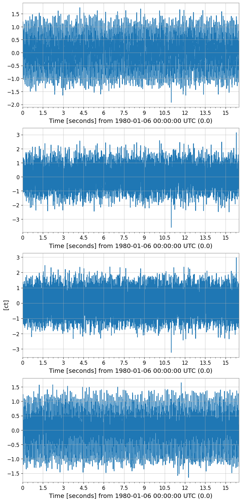
1. Prepare Synthetic Multi-channel Data
We simulate a realistic scenario:
Two hidden sources: a 10 Hz sine wave and broadband noise
Four observed channels: linear mixtures of the hidden sources
This mirrors real-world scenarios in gravitational-wave detectors where physical signals are mixed across multiple sensor channels.
[3]:
rng = np.random.default_rng(42)
fs = 512 # sample rate [Hz]
T = 16.0 # duration [s]
n = int(fs * T)
t = np.arange(n) / fs
# Two independent source signals
src1 = np.sin(2 * np.pi * 10.0 * t) # 10 Hz tone
src2 = rng.normal(0, 1, n) # broadband noise
src3 = np.sin(2 * np.pi * 40.0 * t + 0.7) # 40 Hz tone
# Mixing matrix (4 observed channels from 3 sources)
A = np.array([
[0.8, 0.3, 0.1],
[0.4, 0.7, 0.2],
[0.2, 0.5, 0.9],
[0.6, -0.2, 0.5],
])
sources = np.stack([src1, src2, src3], axis=0) # (3, n)
mixed = A @ sources # (4, n)
# Add small instrument noise
mixed += 0.05 * rng.normal(0, 1, mixed.shape)
# Build TimeSeriesMatrix (4 channels × 1 col × n samples)
dt = (1 / fs) * u.s
t0 = 0 * u.s
data_3d = mixed[:, np.newaxis, :] # (4, 1, n)
tsm = TimeSeriesMatrix(
data_3d,
dt=dt,
t0=t0,
units=np.full((4, 1), u.ct),
)
tsm.channel_names = [f"CH{i}" for i in range(4)]
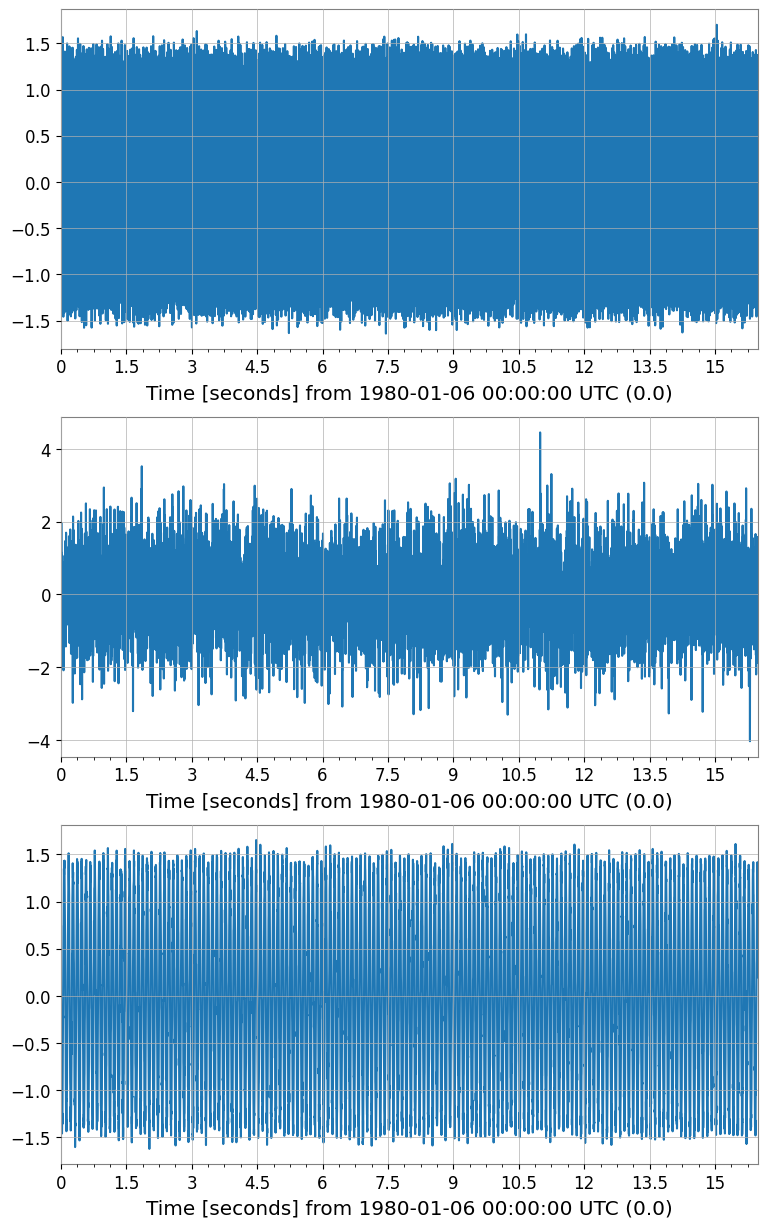
print("TimeSeriesMatrix shape:", tsm.shape) # (4, 1, 8192)
tsm.plot(subplots=True, xscale="seconds");
TimeSeriesMatrix shape: (4, 1, 8192)
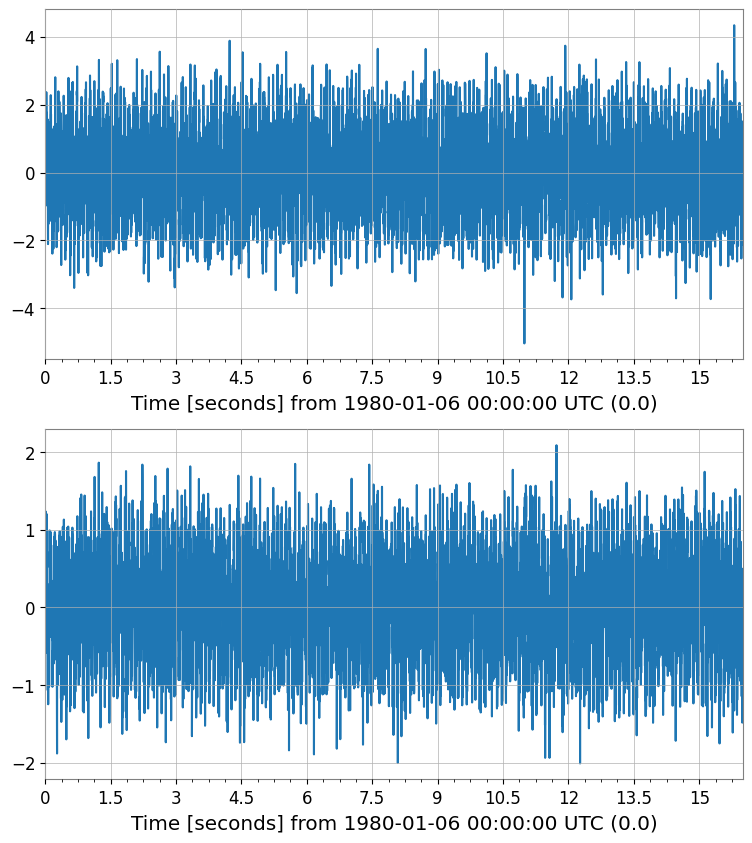
2. PCA – Dimensionality Reduction
TimeSeriesMatrix.pca() returns the score matrix and, optionally, a PCAResult object containing the fitted model.
[4]:
# Fit PCA – keep 2 principal components out of 4 channels
pca_scores, pca_res = tsm.pca(n_components=2, return_model=True)

print("PCA score shape:", pca_scores.shape)           # (2, 1, n)
print("Explained variance ratio:", pca_res.explained_variance_ratio)

pca_scores.plot(subplots=True, xscale="seconds");
PCA score shape: (2, 1, 8192)
Explained variance ratio: [0.68552389 0.18734173]
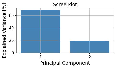
[5]:
# Visualize explained variance (scree plot)
fig, ax = plt.subplots(figsize=(5, 3))

evr = pca_res.explained_variance_ratio
ax.bar(range(1, len(evr) + 1), evr * 100, color="steelblue")
ax.set_xlabel("Principal Component")
ax.set_ylabel("Explained Variance [%]")
ax.set_title("Scree Plot")
ax.set_xticks(range(1, len(evr) + 1))
plt.tight_layout()
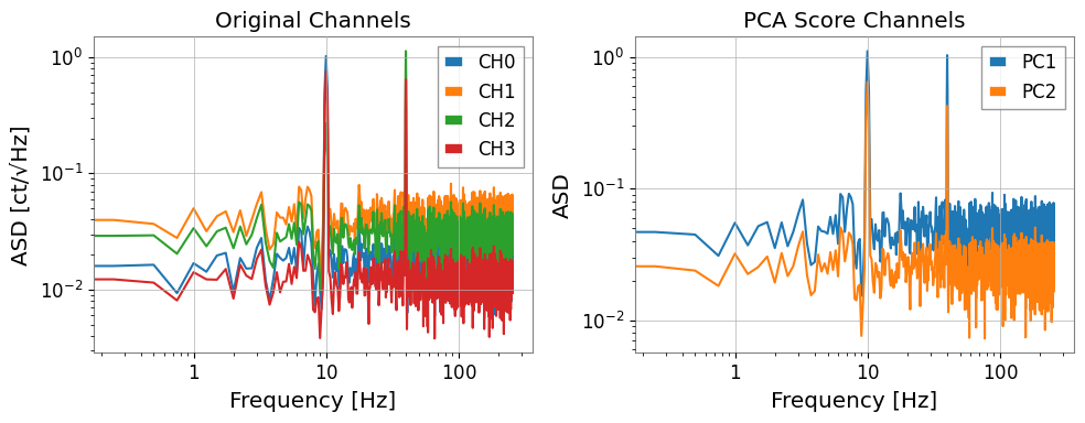
[6]:
# Compare ASD of original channels vs PC scores
fig, axes = plt.subplots(1, 2, figsize=(10, 4))

asd_orig = tsm.asd(fftlength=4, overlap=0.5)
for i in range(asd_orig.shape[0]):
    axes[0].loglog(
        asd_orig[i, 0].frequencies.value,
        asd_orig[i, 0].value,
        label=f"CH{i}",
    )
axes[0].set_xlabel("Frequency [Hz]")
axes[0].set_ylabel("ASD [ct/√Hz]")
axes[0].set_title("Original Channels")
axes[0].legend()

asd_pca = pca_scores.asd(fftlength=4, overlap=0.5)
for i in range(asd_pca.shape[0]):
    axes[1].loglog(
        asd_pca[i, 0].frequencies.value,
        asd_pca[i, 0].value,
        label=f"PC{i+1}",
    )
axes[1].set_xlabel("Frequency [Hz]")
axes[1].set_ylabel("ASD")
axes[1].set_title("PCA Score Channels")
axes[1].legend()

plt.tight_layout()
3. ICA – Blind Source Separation
TimeSeriesMatrix.ica() runs FastICA and returns a source matrix.
Unlike PCA (which finds directions of maximum variance), ICA finds statistically independent sources — making it more suitable for separating physically distinct noise contributions.
[7]:
# Fit ICA – recover 3 independent components
ica_sources = tsm.ica(n_components=3, random_state=0)

print("ICA source shape:", ica_sources.shape)   # (3, 1, n)

ica_sources.plot(subplots=True, xscale="seconds");
ICA source shape: (3, 1, 8192)
[8]:
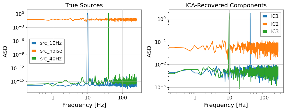
# Compare ICA sources vs. known sources in frequency domain
fig, axes = plt.subplots(1, 2, figsize=(10, 4))

# True sources (for reference)
src_3d = np.stack([src1, src2, src3], axis=0)[:, np.newaxis, :]  # (3,1,n)
tsm_src = TimeSeriesMatrix(src_3d, dt=dt, t0=t0)
tsm_src.channel_names = ["src_10Hz", "src_noise", "src_40Hz"]
asd_src = tsm_src.asd(fftlength=4, overlap=0.5)

for i in range(3):
    axes[0].loglog(
        asd_src[i, 0].frequencies.value,
        asd_src[i, 0].value,
        label=tsm_src.channel_names[i],
    )
axes[0].set_title("True Sources")
axes[0].set_xlabel("Frequency [Hz]")
axes[0].set_ylabel("ASD")
axes[0].legend()

asd_ica = ica_sources.asd(fftlength=4, overlap=0.5)
for i in range(asd_ica.shape[0]):
    axes[1].loglog(
        asd_ica[i, 0].frequencies.value,
        asd_ica[i, 0].value,
        label=f"IC{i+1}",
    )
axes[1].set_title("ICA-Recovered Components")
axes[1].set_xlabel("Frequency [Hz]")
axes[1].set_ylabel("ASD")
axes[1].legend()

plt.tight_layout()
4. Preprocessing: Standardization and Whitening
ICA (and PCA) require data to be scaled appropriately. TimeSeriesMatrix provides built-in preprocessing:
Method |
Description |
|---|---|
|
Zero mean, unit variance per channel |
|
Median / MAD scaling (robust to outliers) |
|
PCA whitening – decorrelates channels |
The pca() and ica() methods accept a scale parameter to apply these internally.
[9]:
# Manual preprocessing pipeline
tsm_z = tsm.standardize(method='zscore')

print("Mean  ≈ 0:", np.allclose(tsm_z.value.mean(axis=-1), 0, atol=1e-10))
print("Std   ≈ 1:", np.allclose(tsm_z.value.std(axis=-1),  1, atol=0.01))

# ICA with internal z-score scaling
ica_scaled = tsm.ica(n_components=3, scale='zscore', random_state=0)
print("ICA (with zscore) shape:", ica_scaled.shape)

# PCA with robust scaling
pca_robust, pca_res2 = tsm.pca(n_components=2, scale='robust', return_model=True)
print("PCA (robust) EVR:", pca_res2.explained_variance_ratio)
Mean  ≈ 0: True
Std   ≈ 1: True
ICA (with zscore) shape: (3, 1, 8192)
PCA (robust) EVR: [0.44248267 0.37626797]
5. Handling Missing Values (NaN)
Real detector data often contains gaps. Use nan_policy='impute' to handle NaNs before decomposition.
[10]:
# Inject some NaN gaps (simulating data gaps)
tsm_nan = tsm.copy()
tsm_nan.value[0, 0, 100:120] = np.nan
tsm_nan.value[2, 0, 500:510] = np.nan

print("NaN count:", np.sum(np.isnan(tsm_nan.value)))

# PCA with linear interpolation of NaN gaps
pca_nanfill, _ = tsm_nan.pca(
    n_components=2,
    nan_policy='impute',
    impute_kwargs={'method': 'interpolate'},
    return_model=True,
)
print("PCA (nan impute) shape:", pca_nanfill.shape)
NaN count: 30
PCA (nan impute) shape: (2, 1, 8192)
6. Migration from scikit-learn
Before (scikit-learn directly):
from sklearn.decomposition import PCA, FastICA
import numpy as np

# Raw numpy array: (n_samples, n_features)
X = data.reshape(n_channels, n_samples).T  # (n_samples, n_channels)

pca = PCA(n_components=2)
scores = pca.fit_transform(X)           # (n_samples, 2)

ica = FastICA(n_components=3, random_state=0)
sources = ica.fit_transform(X)          # (n_samples, 3)
After (gwexpy):
# TimeSeriesMatrix preserves dt/t0/units throughout
pca_scores, pca_res = tsm.pca(n_components=2, return_model=True)
ica_sources          = tsm.ica(n_components=3, random_state=0)
The gwexpy API automatically:
Preserves time axis (
dt,t0,times) in the output matrixKeeps unit metadata
Provides direct plotting via
.plot()Handles NaN policies and scaling internally
Summary
Method |
Key parameters |
Output |
|---|---|---|
|
|
|
|
|
|
Both methods return TimeSeriesMatrix objects, so all downstream operations (.plot(), .asd(), .coherence()) work without any additional conversion.
See also: