Note

This page was generated from a Jupyter Notebook. Download the notebook (.ipynb)

FrequencySeriesMatrix Tutorial

FrequencySeriesMatrix is a 3-dimensional array container that extends SeriesMatrix for the frequency domain (FrequencySeries) with shape: Nrow × Ncol × Nfreq.

• FrequencySeries-compatible aliases such as df / f0 / frequencies

• Element access returns FrequencySeries (fsm[i, j])

• Filter application (magnitude-only: filter) and complex response application (apply_response)

• Conversion to time-domain TimeSeriesMatrix via ifft()

• Direct use of display methods (plot, step, repr, _repr_html_)

In this notebook, we do not define additional utility functions; instead, we directly call class methods to verify their behavior.

import matplotlib.pyplot as plt
import numpy as np
from astropy import units as u

from gwexpy.frequencyseries import FrequencySeries, FrequencySeriesMatrix
from gwexpy.timeseries import TimeSeriesMatrix

plt.rcParams.update({"figure.figsize": (5, 3), "axes.grid": True})

Prepare Representative Data

We calculate fft/asd from TimeSeriesMatrix to obtain FrequencySeriesMatrix.

rng = np.random.default_rng(0)

n = 1024
dt = (1 / 256) * u.s
t0 = 0 * u.s
t = (np.arange(n) * dt).to_value(u.s)

tone10 = np.sin(2 * np.pi * 10 * t)
tone20 = np.sin(2 * np.pi * 20 * t + 0.3)

data = np.empty((2, 2, n), dtype=float)
data[0, 0] = 0.5 * tone10 + 0.05 * rng.normal(size=n)
data[0, 1] = 0.5 * tone20 + 0.05 * rng.normal(size=n)
data[1, 0] = 0.3 * tone10 + 0.3 * tone20 + 0.05 * rng.normal(size=n)
data[1, 1] = 0.2 * tone10 - 0.4 * tone20 + 0.05 * rng.normal(size=n)

units = np.full((2, 2), u.V)
names = [["ch00", "ch01"], ["ch10", "ch11"]]
channels = [["X:A", "X:B"], ["Y:A", "Y:B"]]

tsm = TimeSeriesMatrix(
    data,
    dt=dt,
    t0=t0,
    units=units,
    names=names,
    channels=channels,
    rows={"r0": {"name": "row0"}, "r1": {"name": "row1"}},
    cols={"c0": {"name": "col0"}, "c1": {"name": "col1"}},
    name="demo",
)

fft = tsm.fft()
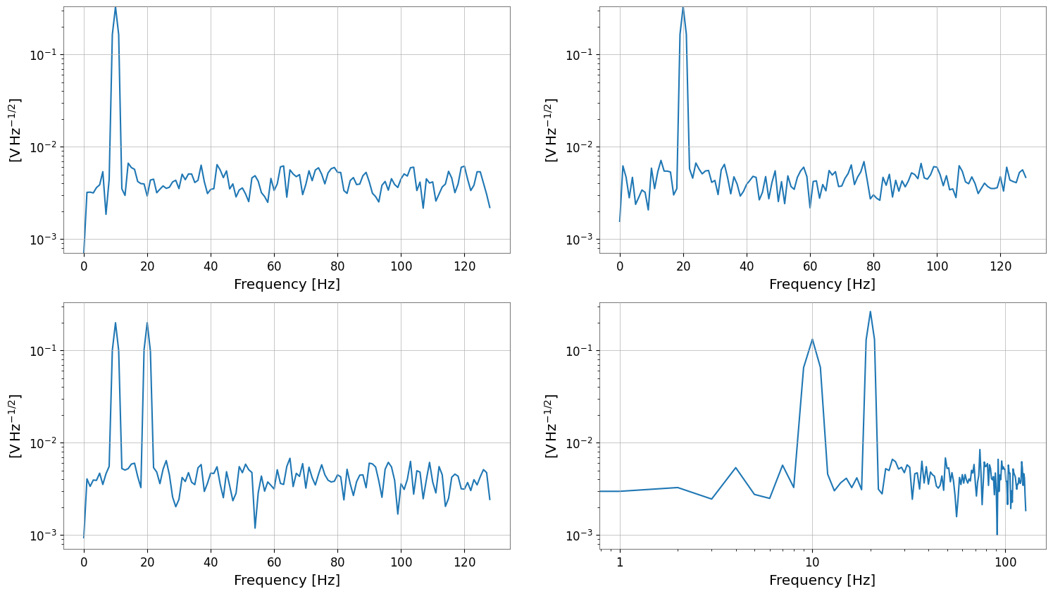
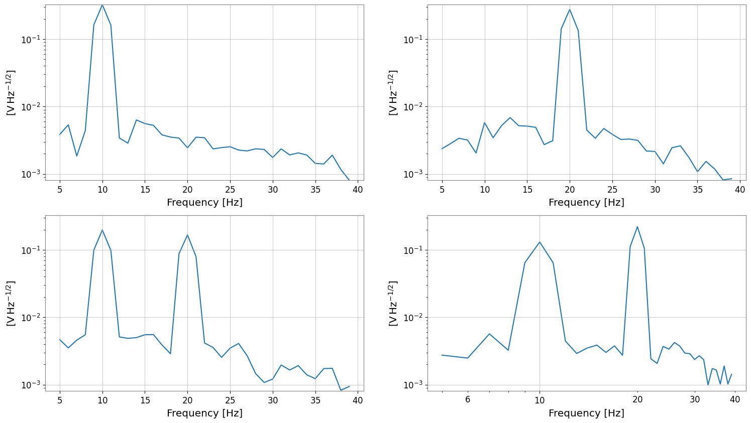
asd = tsm.asd(fftlength=1, overlap=0.5)

print("tsm", tsm.shape, "sample_rate", tsm.sample_rate)
print("fft", fft.shape, "df", fft.df, "f0", fft.f0)
print("asd", asd.shape, "unit", asd[0, 0].unit)
print("frequencies[:5]", asd.frequencies[:5])

display(asd)
asd.plot(subplots=True)
plt.xscale("log")
plt.yscale("log")

tsm (2, 2, 1024) sample_rate 256.0 Hz
fft (2, 2, 513) df 0.25 Hz f0 0.0 Hz
asd (2, 2, 129) unit V / Hz(1/2)
frequencies[:5] [0. 1. 2. 3. 4.] Hz

SeriesMatrix: shape=(2, 2, 129), name='demo'

• epoch: 0.0 s
• x0: 0.0 Hz, dx: 1.0 Hz, N_samples: 129
• xunit: Hz

Row Metadata

	name	channel	unit
key
r0	row0
r1	row1

Column Metadata

	name	channel	unit
key
c0	col0
c1	col1

Element Metadata

	unit	name	channel	row	col
0	V / Hz(1/2)	ch00	X:A	0	0
1	V / Hz(1/2)	ch01	X:B	0	1
2	V / Hz(1/2)	ch10	Y:A	1	0
3	V / Hz(1/2)	ch11	Y:B	1	1

Various Input Patterns (Constructor Examples)

We verify inputs via df/f0, frequencies, 2D list of FrequencySeries, Quantity input, etc.

print("=== FrequencySeriesMatrix Constructor Examples ===")

freqs = np.linspace(0, 64, 65) * u.Hz
f = freqs.to_value(u.Hz)

peak10 = np.exp(-0.5 * ((f - 10) / 1.5) ** 2)
peak20 = np.exp(-0.5 * ((f - 20) / 2.0) ** 2)

data_f = np.empty((2, 2, len(freqs)), dtype=float)
data_f[0, 0] = peak10
data_f[0, 1] = peak20
data_f[1, 0] = 0.6 * peak10 + 0.4 * peak20
data_f[1, 1] = 0.2 * peak10 - 0.5 * peak20

units_f = np.full((2, 2), u.V / u.Hz**0.5)
names_f = [["p10", "p20"], ["mix", "diff"]]
channels_f = [["X:A", "X:B"], ["Y:A", "Y:B"]]

# Case 1: Explicitly specify frequencies
fsm = FrequencySeriesMatrix(
    data_f,
    frequencies=freqs,
    units=units_f,
    names=names_f,
    channels=channels_f,
    rows={"r0": {"name": "row0"}, "r1": {"name": "row1"}},
    cols={"c0": {"name": "col0"}, "c1": {"name": "col1"}},
    name="peaks",
)
print("case1 frequencies", fsm.shape, "df", fsm.df, "f0", fsm.f0)

# Case 2: Specify df/f0 (axis generated via Index.define)
fsm_df = FrequencySeriesMatrix(
    data_f, df=1 * u.Hz, f0=0 * u.Hz, units=units_f, names=names_f
)
print("case2 df/f0", fsm_df.shape, "df", fsm_df.df)

# Case 3: Construct from 2D list of FrequencySeries
fs00 = FrequencySeries(
    data_f[0, 0], frequencies=freqs, unit=units_f[0, 0], name="p10", channel="X:A"
)
fs01 = FrequencySeries(
    data_f[0, 1], frequencies=freqs, unit=units_f[0, 1], name="p20", channel="X:B"
)
fs10 = FrequencySeries(
    data_f[1, 0], frequencies=freqs, unit=units_f[1, 0], name="mix", channel="Y:A"
)
fs11 = FrequencySeries(
    data_f[1, 1], frequencies=freqs, unit=units_f[1, 1], name="diff", channel="Y:B"
)
fsm_from_fs = FrequencySeriesMatrix([[fs00, fs01], [fs10, fs11]])
print(
    "case3 from FrequencySeries",
    fsm_from_fs.shape,
    "cell type",
    type(fsm_from_fs[0, 0]),
)

# Case 4: Quantity input (units set automatically)
fsm_q = FrequencySeriesMatrix(data_f * (u.mV / u.Hz**0.5), frequencies=freqs)
print("case4 Quantity meta unit", fsm_q.meta[0, 0].unit)

# Case 5: Irregular frequencies
irreg = np.array([0, 1, 2, 4, 8]) * u.Hz
fsm_irreg = FrequencySeriesMatrix(
    np.ones((1, 1, len(irreg))), frequencies=irreg, units=[[u.V]], names=[["irreg"]]
)
print("case5 irregular frequencies", fsm_irreg.frequencies)

=== FrequencySeriesMatrix Constructor Examples ===
case1 frequencies (2, 2, 65) df 1.0 Hz f0 0.0 Hz
case2 df/f0 (2, 2, 65) df 1.0 Hz
case3 from FrequencySeries (2, 2, 65) cell type <class 'gwexpy.frequencyseries.frequencyseries.FrequencySeries'>
case4 Quantity meta unit mV / Hz(1/2)
case5 irregular frequencies [0. 1. 2. 4. 8.] Hz

Indexing and Slicing

• fsm[i, j] returns a FrequencySeries

• Slicing returns a FrequencySeriesMatrix

• Access is also possible using row/col labels

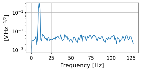
s00 = asd[0, 0]
print("[0,0]", "type", type(s00), "df", s00.df, "f0", s00.f0, "unit", s00.unit)
print("[0,0]", "name", s00.name, "channel", s00.channel)
s00.plot()

s01 = asd["r0", "c1"]
print("[r0,c1]", "name", s01.name, "channel", s01.channel)

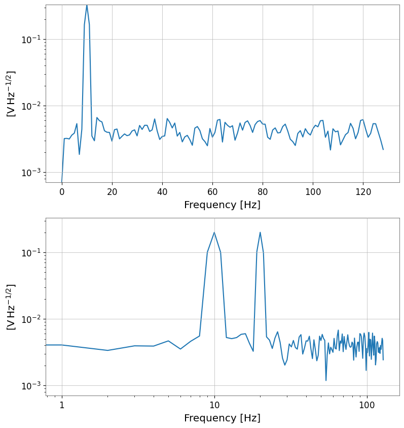
sub = asd[:, 0]
print("asd[:,0] ->", type(sub), sub.shape)
sub.plot(subplots=True)
plt.xscale("log")
plt.yscale("log")

[0,0] type <class 'gwexpy.frequencyseries.frequencyseries.FrequencySeries'> df 1.0 Hz f0 0.0 Hz unit V / Hz(1/2)
[0,0] name ch00 channel X:A
[r0,c1] name ch01 channel X:B
asd[:,0] -> <class 'gwexpy.frequencyseries.matrix.FrequencySeriesMatrix'> (2, 1, 129)

Sample Axis Editing (frequency axis)

• diff / pad return a FrequencySeriesMatrix

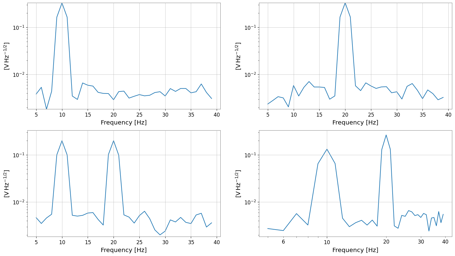
band = asd.crop(start=5 * u.Hz, end=40 * u.Hz)
print("band", type(band), band.shape, "span", band.xspan)
band.plot(subplots=True)
plt.xscale("log")
plt.yscale("log")

diffed = band.diff(n=1)
print("diffed", type(diffed), diffed.shape, "df", diffed.df)

padded = band.pad(5)
print("padded", type(padded), padded.shape, "f0", padded.f0)

band <class 'gwexpy.frequencyseries.matrix.FrequencySeriesMatrix'> (2, 2, 35) span (<Quantity 5. Hz>, <Quantity 40. Hz>)
diffed <class 'gwexpy.frequencyseries.matrix.FrequencySeriesMatrix'> (2, 2, 34) df 1.0 Hz
padded <class 'gwexpy.frequencyseries.matrix.FrequencySeriesMatrix'> (2, 2, 45) f0 0.0 Hz

Operations (ufunc / apply_response)

• Ufunc operations such as scalar multiplication preserve units

• apply_response is an extended method to apply complex/real frequency responses (dimensionless)

scaled = 2 * band
print("scaled unit", scaled[0, 0].unit)

# Simple real response suppressing around 30 Hz
resp_mag = 1 / (1 + (band.frequencies / (30 * u.Hz)) ** 4)
shaped = band.apply_response(resp_mag)
print(
    "apply_response",
    shaped.shape,
    "dtype",
    shaped.value.dtype,
    "unit",
    shaped[0, 0].unit,
)

shaped.plot(subplots=True)
plt.xscale("log")
plt.yscale("log")

scaled unit V / Hz(1/2)
apply_response (2, 2, 35) dtype float64 unit V / Hz(1/2)

filter (magnitude-only)

filter delegates to GWpy’s fdfilter, applying the filter’s “magnitude response” only (not the phase).

As an example, we apply an IIR filter created with scipy.signal.butter to the fft and then convert back to the time domain with ifft().

from scipy import signal

sr = tsm.sample_rate.to_value(u.Hz)
b, a = signal.butter(4, [5, 40], btype="bandpass", fs=sr)

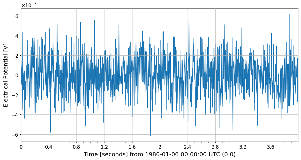
fft_filt = fft.filter(b, a, analog=False)
tsm_filt = fft_filt.ifft()

print("fft_filt", fft_filt.shape, "df", fft_filt.df)
print("tsm_filt", tsm_filt.shape, "dt", tsm_filt.dt)

tsm_filt[0, 0].plot(xscale="seconds");

fft_filt (2, 2, 513) df 0.25 Hz
tsm_filt (2, 2, 1024) dt 0.00390625 s

ifft (FFT to Time Domain)

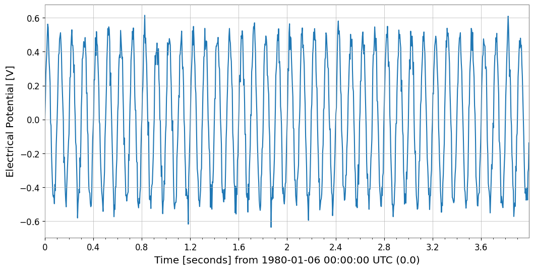
Applying ifft() to the output of TimeSeriesMatrix.fft() reproduces the original TimeSeriesMatrix (within numerical precision).

tsm_back = fft.ifft()
rms = np.sqrt(np.mean((tsm_back[0, 0].value - tsm[0, 0].value) ** 2))
print("ifft back", tsm_back.shape, "dt", tsm_back.dt, "t0", tsm_back.t0)
print("rms error (cell 0,0)", rms)

tsm[0, 0].plot(xscale="seconds")
tsm_back[0, 0].plot(xscale="seconds");

ifft back (2, 2, 1024) dt 0.00390625 s t0 0.0 s
rms error (cell 0,0) 8.131556499372449e-17

Display Methods: repr / plot / step

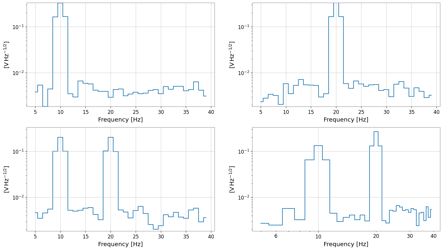
• repr: Text representation

• _repr_html_: In notebooks, display(fsm) shows tabular format

• plot / step: Class methods for direct plotting (not saved)

print("repr:\n", band)
display(band)

band.plot(subplots=True)
plt.xscale("log")
plt.yscale("log")

band.step(where="mid")
plt.xscale("log")
plt.yscale("log")

repr:
 SeriesMatrix(shape=(2, 2, 35),  name='demo')
  epoch   : 0.0 s
  x0      : 5.0 Hz
  dx      : 1.0 Hz
  xunit   : Hz
  samples : 35

[ Row metadata ]
     name channel unit
key
r0   row0
r1   row1

[ Column metadata ]
     name channel unit
key
c0   col0
c1   col1

[ Elements metadata ]
          unit  name channel  row  col
0  V / Hz(1/2)  ch00     X:A    0    0
1  V / Hz(1/2)  ch01     X:B    0    1
2  V / Hz(1/2)  ch10     Y:A    1    0
3  V / Hz(1/2)  ch11     Y:B    1    1

SeriesMatrix: shape=(2, 2, 35), name='demo'

• epoch: 0.0 s
• x0: 5.0 Hz, dx: 1.0 Hz, N_samples: 35
• xunit: Hz

Row Metadata

	name	channel	unit
key
r0	row0
r1	row1

Column Metadata

	name	channel	unit
key
c0	col0
c1	col1

Element Metadata

	unit	name	channel	row	col
0	V / Hz(1/2)	ch00	X:A	0	0
1	V / Hz(1/2)	ch01	X:B	0	1
2	V / Hz(1/2)	ch10	Y:A	1	0
3	V / Hz(1/2)	ch11	Y:B	1	1

Summary

• FrequencySeriesMatrix allows batch processing as a matrix while preserving the frequency axis (df/f0/frequencies) and element metadata.

• filter applies magnitude-only filtering, while apply_response can apply arbitrary frequency responses including complex responses.

• Using ifft(), you can convert back to the time-domain TimeSeriesMatrix, enabling workflows where processing is done in the frequency domain and then verified as waveforms.