Note

This page was generated from a Jupyter Notebook. Download the notebook (.ipynb)

TimeSeriesMatrix Tutorial

TimeSeriesMatrix is a 3-dimensional array container that extends SeriesMatrix for TimeSeries (shape: Nrow × Ncol × Nsample).

• TimeSeries-compatible aliases such as dt / t0 / times

• Element access returns TimeSeries (tsm[i, j])

• Time-domain processing (detrend/bandpass/resample …) applied element-wise

• Spectral analysis such as FFT/PSD/ASD and coherence (returns FrequencySeriesMatrix)

• Display methods (plot, step, repr, _repr_html_) work out of the box

In this notebook, we do not define additional utility functions but directly call class methods to verify their behavior.

import matplotlib.pyplot as plt
import numpy as np
from astropy import units as u

from gwexpy.timeseries import TimeSeries, TimeSeriesMatrix

Prepare Representative Data

• Create a 2×2 TimeSeriesMatrix and check dt/t0/times and metadata (unit/name/channel).

rng = np.random.default_rng(0)

# Sample configuration
n = 1024
dt = (1 / 256) * u.s
t0 = 0 * u.s

t = (np.arange(n) * dt).to_value(u.s)

tone10 = np.sin(2 * np.pi * 10 * t)
tone20 = np.sin(2 * np.pi * 20 * t + 0.3)

data = np.empty((2, 2, n), dtype=float)
data[0, 0] = 0.5 * tone10 + 0.05 * rng.normal(size=n)
data[0, 1] = 0.5 * tone20 + 0.05 * rng.normal(size=n)
data[1, 0] = 0.3 * tone10 + 0.3 * tone20 + 0.05 * rng.normal(size=n)
data[1, 1] = 0.2 * tone10 - 0.4 * tone20 + 0.05 * rng.normal(size=n)

units = np.full((2, 2), u.V)
names = [["ch00", "ch01"], ["ch10", "ch11"]]
channels = [["X:A", "X:B"], ["Y:A", "Y:B"]]

tsm = TimeSeriesMatrix(
    data,
    dt=dt,
    t0=t0,
    units=units,
    names=names,
    channels=channels,
    rows={"r0": {"name": "row0"}, "r1": {"name": "row1"}},
    cols={"c0": {"name": "col0"}, "c1": {"name": "col1"}},
    name="demo",
)

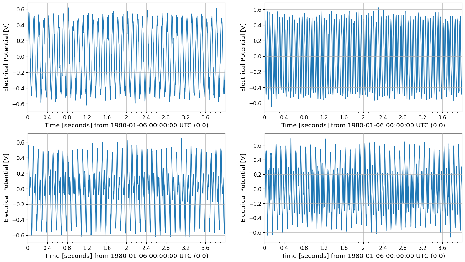
display(tsm)
tsm.plot();

SeriesMatrix: shape=(2, 2, 1024), name='demo'

• epoch: 0.0 s
• x0: 0.0 s, dx: 0.00390625 s, N_samples: 1024
• xunit: s

Row Metadata

	name	channel	unit
key
r0	row0
r1	row1

Column Metadata

	name	channel	unit
key
c0	col0
c1	col1

Element Metadata

	unit	name	channel	row	col
0	V	ch00	X:A	0	0
1	V	ch01	X:B	0	1
2	V	ch10	Y:A	1	0
3	V	ch11	Y:B	1	1

Various Input Patterns (Constructor Examples)

In addition to dt/t0, we verify sample_rate or times, 2D lists of TimeSeries, Quantity input, etc.

print("=== TimeSeriesMatrix Constructor Examples ===")
times = tsm.times

# Case 1: Specify sample_rate (instead of dt)
tsm_sr = TimeSeriesMatrix(
    data,
    sample_rate=256 * u.Hz,
    t0=t0,
    units=units,
    names=names,
    channels=channels,
)
print("case1 sample_rate", "dt", tsm_sr.dt, "sample_rate", tsm_sr.sample_rate)

# Case 2: Specify times (also supports irregular sampling)
tsm_times = TimeSeriesMatrix(data, times=times, units=units, names=names)
print("case2 times", "dt", tsm_times.dt, "t0", tsm_times.t0, "N", tsm_times.N_samples)

# Case 3: Construct from a 2D list of TimeSeries
ts00 = TimeSeries(data[0, 0], times=times, unit=u.V, name="ch00", channel="X:A")
ts01 = TimeSeries(data[0, 1], times=times, unit=u.V, name="ch01", channel="X:B")
ts10 = TimeSeries(data[1, 0], times=times, unit=u.V, name="ch10", channel="Y:A")
ts11 = TimeSeries(data[1, 1], times=times, unit=u.V, name="ch11", channel="Y:B")
tsm_from_ts = TimeSeriesMatrix([[ts00, ts01], [ts10, ts11]])
print("case3 from TimeSeries", tsm_from_ts.shape, "dt", tsm_from_ts.dt)

# Case 4: Quantity input (units are automatically set)
tsm_q = TimeSeriesMatrix((data * u.mV), dt=dt, t0=t0)
print("case4 Quantity meta unit", tsm_q.meta[0, 0].unit)

# Exception: dt and sample_rate / t0 and epoch cannot be specified simultaneously
for kwargs in [
    dict(dt=dt, sample_rate=256 * u.Hz, t0=t0),
    dict(dt=dt, t0=t0, epoch=t0),
]:
    try:
        _ = TimeSeriesMatrix(data, **kwargs)
    except Exception as e:
        print("error", kwargs, "->", type(e).__name__, e)

=== TimeSeriesMatrix Constructor Examples ===
case1 sample_rate dt 0.00390625 s sample_rate 256.0 Hz
case2 times dt 0.00390625 s t0 0.0 s N 1024
case3 from TimeSeries (2, 2, 1024) dt 0.00390625 s
case4 Quantity meta unit mV
error {'dt': <Quantity 0.00390625 s>, 'sample_rate': <Quantity 256. Hz>, 't0': <Quantity 0. s>} -> ValueError give only one of sample_rate or dt
error {'dt': <Quantity 0.00390625 s>, 't0': <Quantity 0. s>, 'epoch': <Quantity 0. s>} -> ValueError give only one of epoch or t0

Indexing and Slicing

• tsm[i, j] returns a TimeSeries

• Slicing returns a TimeSeriesMatrix

• Can also access via row/col labels

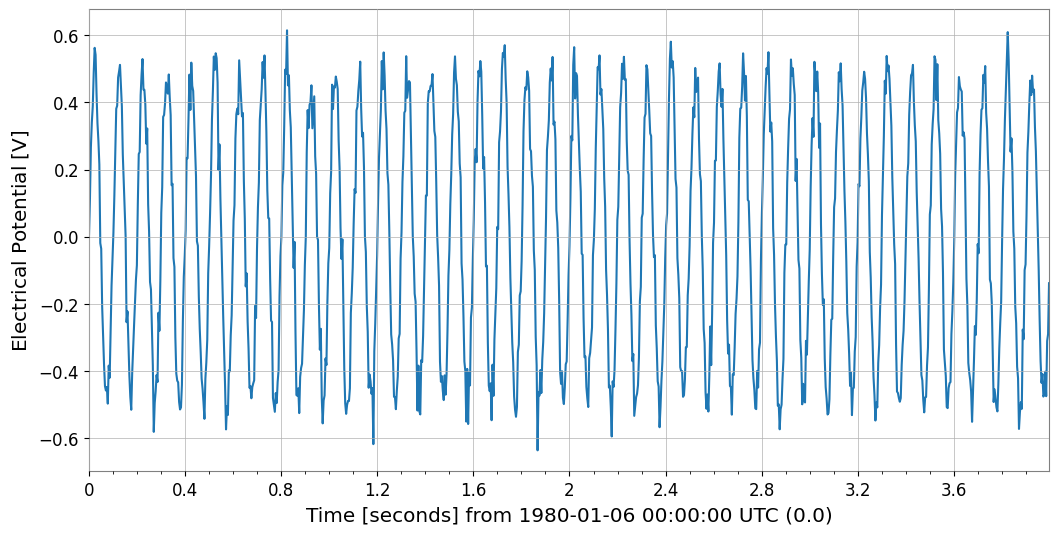
s00 = tsm[0, 0]
print("[0,0]", "type", type(s00), "dt", s00.dt, "t0", s00.t0, "unit", s00.unit)
print("[0,0]", "name", s00.name, "channel", s00.channel)
s00.plot(xscale="seconds")

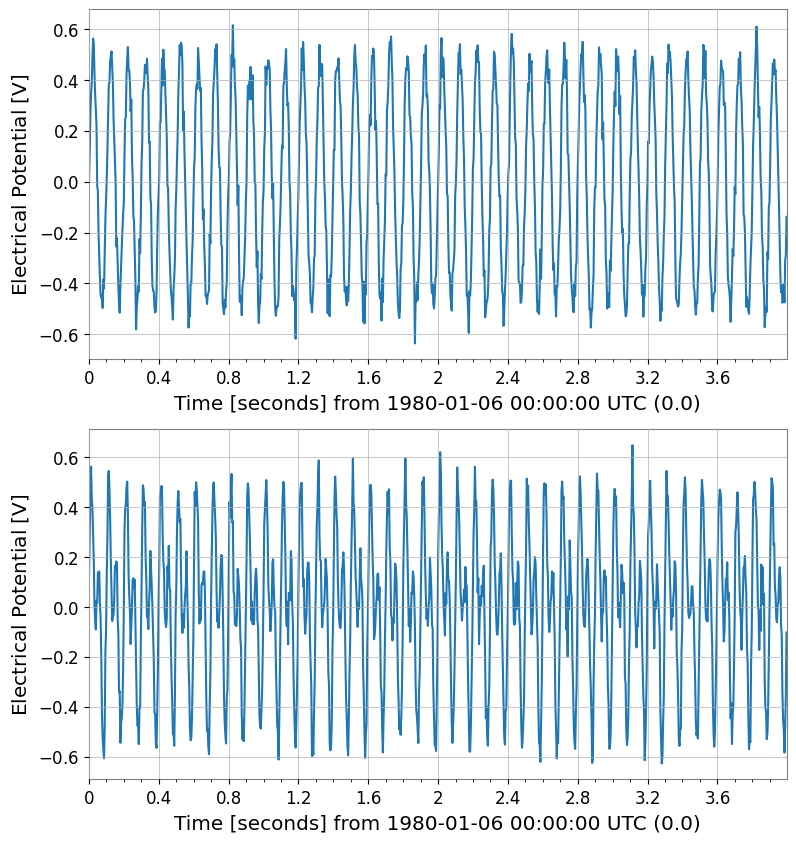
s01 = tsm["r0", "c1"]
print("[r0,c1]", "name", s01.name, "channel", s01.channel)

sub = tsm[:, 0]
print("tsm[:,0] ->", type(sub), sub.shape)
sub.plot(subplots=True, xscale="seconds");

[0,0] type <class 'gwexpy.timeseries.timeseries.TimeSeries'> dt 0.00390625 s t0 0.0 s unit V
[0,0] name ch00 channel X:A
[r0,c1] name ch01 channel X:B
tsm[:,0] -> <class 'gwexpy.timeseries.matrix.TimeSeriesMatrix'> (2, 1, 1024)

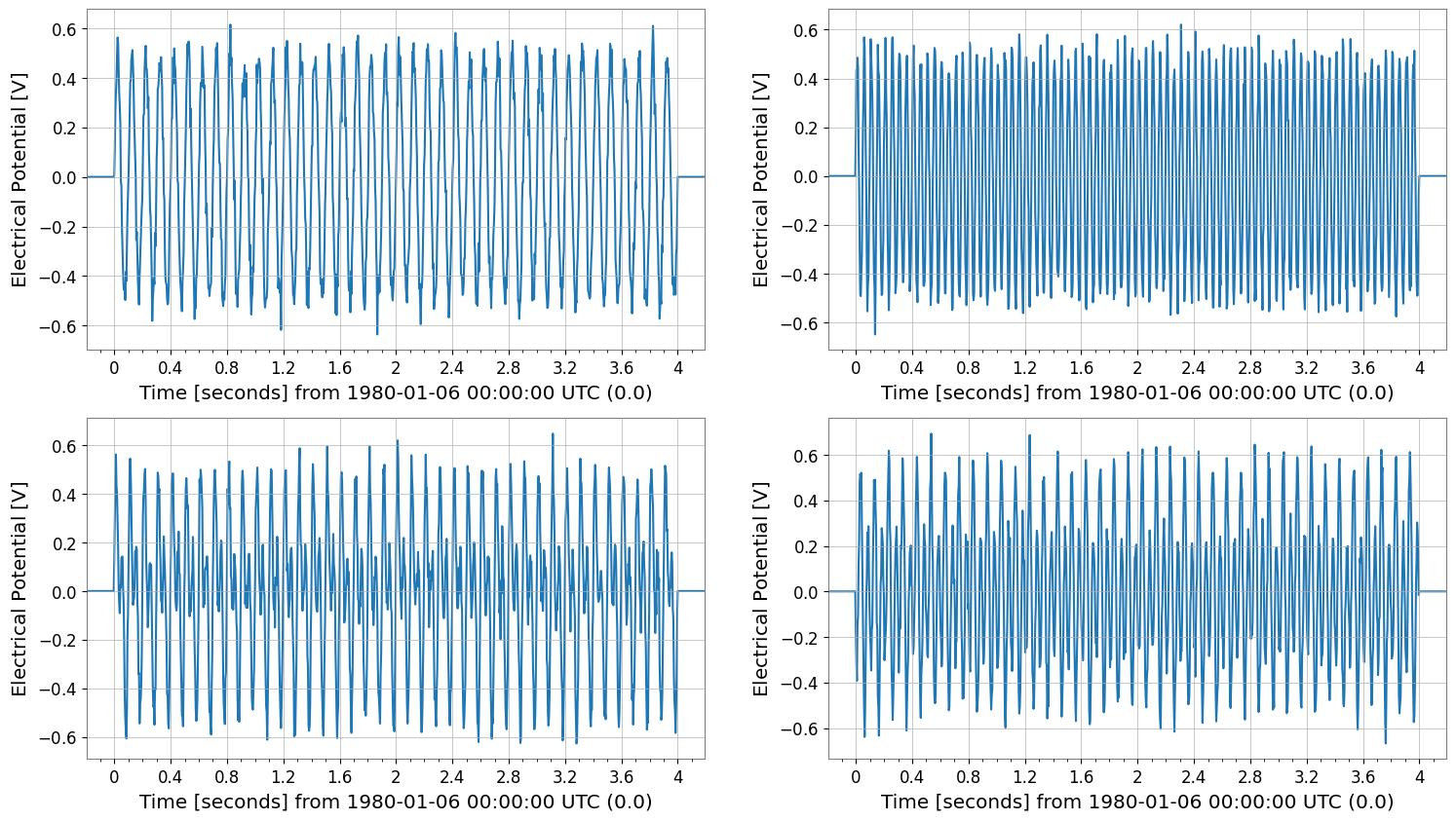
Sample Axis Editing

• diff / pad return TimeSeriesMatrix

• crop currently returns SeriesMatrix, so use view(TimeSeriesMatrix) to restore (contents are the same)

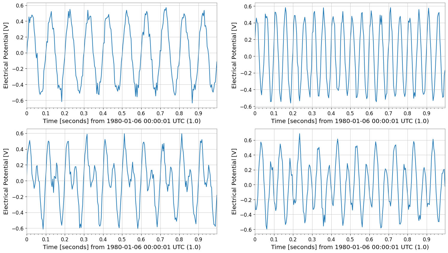
cropped = tsm.crop(start=1 * u.s, end=2 * u.s).view(TimeSeriesMatrix)
print("cropped", type(cropped), cropped.shape, "span", cropped.span)
cropped.plot(subplots=True, xscale="seconds")

diffed = tsm.diff(n=1)
print("diffed", diffed.shape, "dt", diffed.dt)
diffed.plot(subplots=True, xscale="seconds")

padded = tsm.pad(50)
print("padded", padded.shape, "t0", padded.t0)
padded.plot(subplots=True, xscale="seconds");

cropped <class 'gwexpy.timeseries.matrix.TimeSeriesMatrix'> (2, 2, 256) span (<Quantity 1. s>, <Quantity 2. s>)
diffed (2, 2, 1023) dt 0.00390625 s
padded (2, 2, 1124) t0 -0.1953125 s

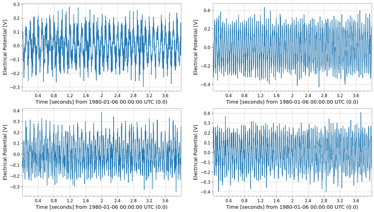
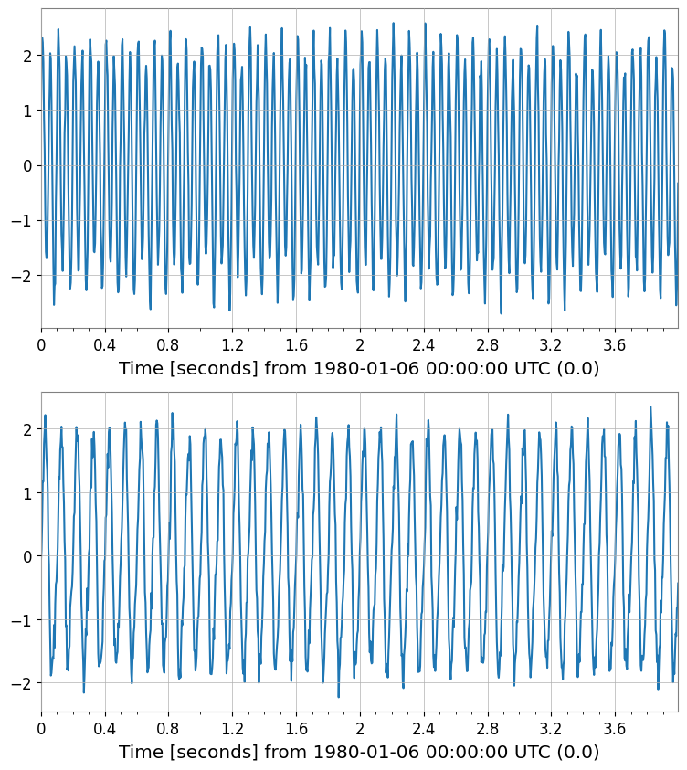
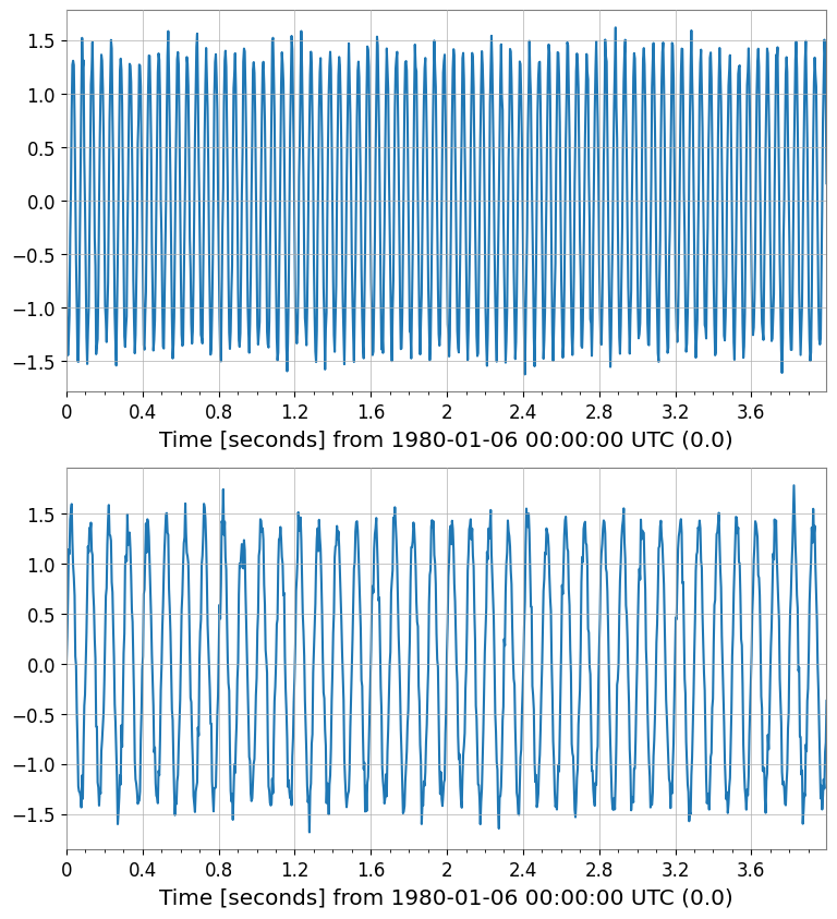
Time-Domain Processing (Element-wise Application of TimeSeries Methods)

TimeSeries methods (detrend, bandpass, resample, etc.) are applied element-wise to the matrix.

detr = tsm.detrend("constant")
bp = detr.bandpass(5, 40)
rs = bp.resample(128)

print("original", tsm.shape, "sample_rate", tsm.sample_rate)
print("bandpass", bp.shape, "sample_rate", bp.sample_rate)
print("resample", rs.shape, "sample_rate", rs.sample_rate)

bp.plot(subplots=True, xscale="seconds")
rs.plot(subplots=True, xscale="seconds");

original (2, 2, 1024) sample_rate 256.0 Hz
bandpass (2, 2, 1024) sample_rate 256.0 Hz
resample (2, 2, 512) sample_rate 128.0 Hz

Missing Value Imputation

Impute missing values (NaN) in the matrix. Applied to each channel separately.

# Create data with missing values (for demo)
tsm_miss = tsm.copy()
# Set some values to NaN in the first channel (note how to access: tsm[0,0] is a time series)
tsm_miss[0, 0].value[50:60] = np.nan

print("Before impute (Has NaN):", np.isnan(tsm_miss[0, 0].value).any())

# Impute (linear interpolation)
tsm_imp = tsm_miss.impute(method="interpolate")
print("After impute (Has NaN):", np.isnan(tsm_imp[0, 0].value).any())

Before impute (Has NaN): False
After impute (Has NaN): False

Preprocessing: Standardization and Whitening

Useful as preprocessing for multivariate analysis.

# Standardize: Scale to mean 0, variance 1
tsm_std = tsm.standardize(method="zscore")

# Whiten: Remove inter-channel correlation (covariance)
# Use PCA to decorrelate
tsm_white, w_model = tsm_std.whiten_channels(return_model=True)

print("Standardized shape:", tsm_std.shape)
print("Whitened shape:", tsm_white.shape)

Standardized shape: (2, 2, 1024)
Whitened shape: (4, 1, 1024)

Decomposition (PCA / ICA)

Efficient dimensionality reduction or source separation.

# Principal Component Analysis (PCA)
# Dimensionality reduction (e.g., 3 channels -> 2 principal components)
n_comp = min(2, tsm.shape[0])
pca_scores, pca_res = tsm_std.pca(n_components=n_comp, return_model=True)

print("PCA Scores shape:", pca_scores.shape)
print("Explained variance ratio:", pca_res.explained_variance_ratio)
pca_scores.plot()
plt.show()
plt.close()

# Independent Component Analysis (ICA)
# Blind Source Separation
ica_sources = tsm_std.ica(n_components=n_comp, random_state=42)
print("ICA Sources shape:", ica_sources.shape)
ica_sources.plot()
plt.show()
plt.close()

PCA Scores shape: (2, 1, 1024)
Explained variance ratio: [0.57128681 0.41742564]

ICA Sources shape: (2, 1, 1024)

Interoperability Introduction

Data can be passed to external libraries such as PyTorch.

try:
    # Convert to PyTorch Tensor
    import torch

    _ = torch
    tensor = tsm.to_torch()
    print("Converted to PyTorch:", tensor.shape)
except ImportError:
    print("PyTorch not installed")

Converted to PyTorch: torch.Size([2, 2, 1024])

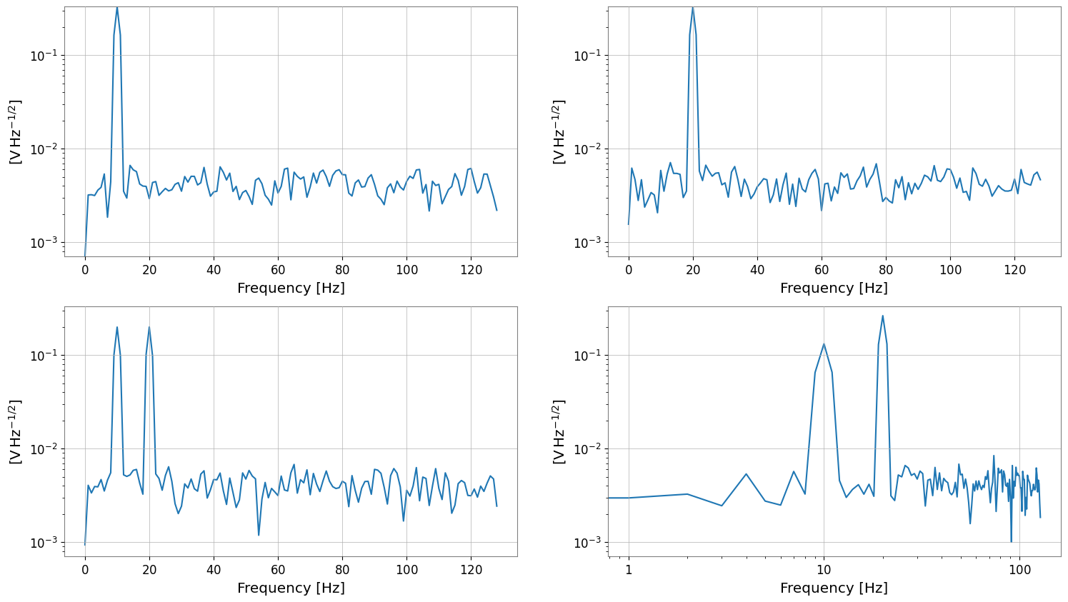
Spectral Analysis (FFT / PSD / ASD)

fft/psd/asd return FrequencySeriesMatrix.

fft = tsm.fft()
print("fft", type(fft), fft.shape, "df", fft.df, "f0", fft.f0)

psd = tsm.psd(fftlength=1, overlap=0.5)
asd = tsm.asd(fftlength=1, overlap=0.5)
print("psd", psd.shape, "unit", psd[0, 0].unit)
print("asd", asd.shape, "unit", asd[0, 0].unit)

asd.plot(subplots=True)
plt.xscale("log")
plt.yscale("log")

fft <class 'gwexpy.frequencyseries.matrix.FrequencySeriesMatrix'> (2, 2, 513) df 0.25 Hz f0 0.0 Hz
psd (2, 2, 129) unit V2 / Hz
asd (2, 2, 129) unit V / Hz(1/2)

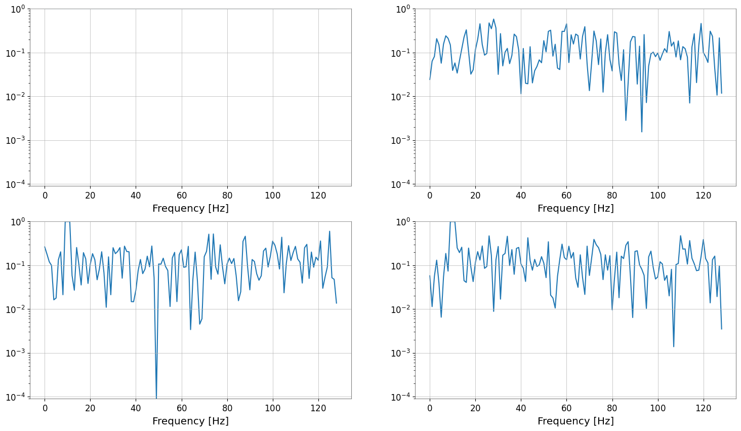
Bivariate Spectral Analysis (Coherence Example)

TimeSeriesMatrix.coherence(other) computes coherence element-wise and returns FrequencySeriesMatrix.

• Passing a TimeSeries as other compares “all elements vs. the same reference”

• Passing a TimeSeriesMatrix as other requires matching shape (Nrow, Ncol)

ref = tsm[0, 0]
coh = tsm.coherence(ref, fftlength=1, overlap=0.5)
print("coherence", type(coh), coh.shape, "unit", coh[0, 0].unit)
coh.plot(subplots=True)

try:
    _ = tsm.coherence(tsm[:, :1], fftlength=1)
except Exception as e:
    print("shape mismatch ->", type(e).__name__, e)

coherence <class 'gwexpy.frequencyseries.matrix.FrequencySeriesMatrix'> (2, 2, 129) unit coherence
shape mismatch -> IndexError index 1 is out of bounds for axis 1 with size 1

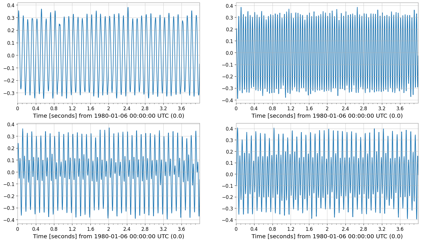
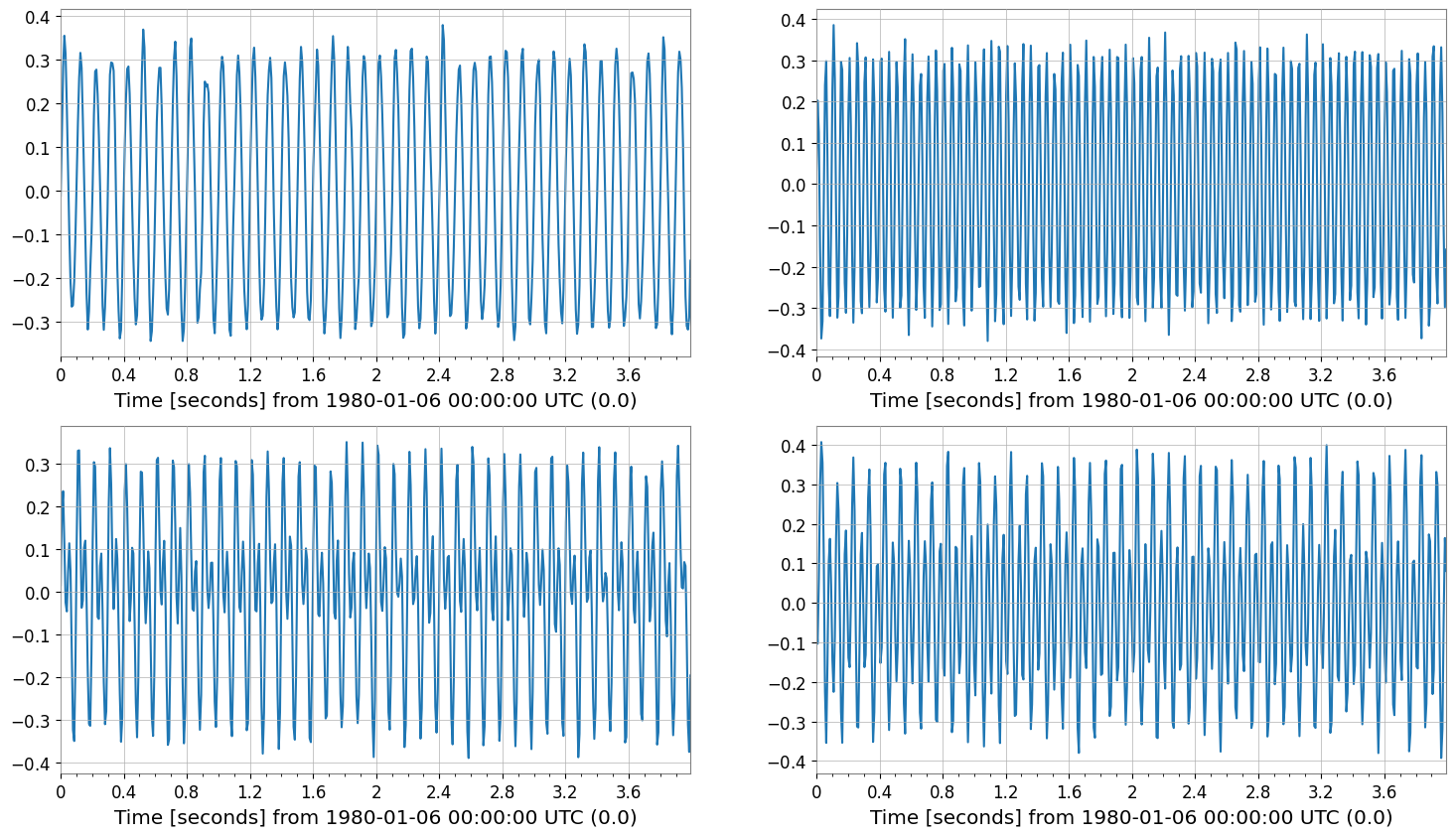
Display Methods: repr / plot / step

• repr: Text display

• _repr_html_: In notebooks, display(tsm) shows a table format

• plot / step: Direct plotting with class methods

print("repr:\n", tsm)
display(tsm)

tsm.plot(subplots=True, xscale="seconds")
tsm.step(where="post", xscale="seconds");

repr:
 SeriesMatrix(shape=(2, 2, 1024),  name='demo')
  epoch   : 0.0 s
  x0      : 0.0 s
  dx      : 0.00390625 s
  xunit   : s
  samples : 1024

[ Row metadata ]
     name channel unit
key
r0   row0
r1   row1

[ Column metadata ]
     name channel unit
key
c0   col0
c1   col1

[ Elements metadata ]
  unit  name channel  row  col
0    V  ch00     X:A    0    0
1    V  ch01     X:B    0    1
2    V  ch10     Y:A    1    0
3    V  ch11     Y:B    1    1

SeriesMatrix: shape=(2, 2, 1024), name='demo'

• epoch: 0.0 s
• x0: 0.0 s, dx: 0.00390625 s, N_samples: 1024
• xunit: s

Row Metadata

	name	channel	unit
key
r0	row0
r1	row1

Column Metadata

	name	channel	unit
key
c0	col0
c1	col1

Element Metadata

	unit	name	channel	row	col
0	V	ch00	X:A	0	0
1	V	ch01	X:B	0	1
2	V	ch10	Y:A	1	0
3	V	ch11	Y:B	1	1

Summary

• TimeSeriesMatrix preserves TimeSeries-compatible axis information (dt/t0/times) and element metadata while enabling batch processing as a matrix.

• Time-domain processing (detrend/bandpass/resample, etc.) and spectral analysis (asd/psd/coherence, etc.) can be applied element-wise in batches.

• First extract a TimeSeries with tsm[i, j] to check behavior, then once familiar, process the entire matrix for convenience.