Note

This page was generated from a Jupyter Notebook. Download the notebook (.ipynb)

# Skipped in CI: Colab/bootstrap dependency install cell.

Case navigation:

• Back to the canonical gallery: Case Studies

• Related reference surfaces: Reference Index, API: Frequency Series, Reference Topics

• Neighboring featured workflows: Noise Budgeting, Active Damping

Tutorial: Transfer Function Measurement

This tutorial demonstrates how to use gwexpy to estimate the transfer function of a system from measured data, fit a physical model to the transfer function, and identify system parameters.

Scenario: We inject white noise into a mechanical vibration system (or electrical circuit) and measure its response. From this input-output data, we will determine the system’s resonance frequency \(f_0\) and quality factor \(Q\).

Workflow:

1. Data generation: Simulate an input signal (white noise) and the system output (resonant system response + measurement noise).

2. Transfer function estimation: Calculate the transfer function and coherence from the input-output time series data and plot the Bode plot.

3. Model fitting: Fit a theoretical model (such as a Lorentzian function) to the estimated transfer function to extract system parameters.

import warnings

warnings.filterwarnings("ignore", category=UserWarning)
warnings.filterwarnings("ignore", category=DeprecationWarning)

import matplotlib.pyplot as plt
import numpy as np
from scipy import signal

from gwexpy import TimeSeries
from gwexpy.plot import Plot

1. Generating Experimental Data (Simulation)

We will conduct a virtual experiment.

• System: Second-order resonant system (harmonic oscillator)

  • Resonance frequency \(f_0 = 300\) Hz

  • Quality factor \(Q = 50\)

• Input: White noise

• Measurement: Sampling frequency 2048 Hz, duration 60 seconds

The output signal will also include measurement noise.

# --- Parameter Settings: choose a resonator whose f0 and Q mimic a narrow mechanical mode worth identifying from measured data. ---
fs = 2048.0  # Sampling frequency [Hz]
duration = 60.0  # Duration [s]
f0_true = 300.0  # True resonance frequency [Hz]
Q_true = 50.0  # True quality factor

# --- Time axis and input signal: broadband drive excites the plant across frequency so the resonance can be measured in one experiment. ---
t = np.linspace(0, duration, int(duration * fs), endpoint=False)
input_data = np.random.normal(0, 1, size=len(t))  # Broadband excitation approximates a swept identification drive without privileging one frequency.

# --- Physical System Simulation (using scipy.signal): this second-order plant stands in for a suspension or actuator resonance. ---
# H(s) uses f0 for the modal frequency and Q for damping width, so fitting them back out tests whether the measurement preserves the true mode shape.
w0 = 2 * np.pi * f0_true
num = [w0**2]
den = [1, w0 / Q_true, w0**2]
system = signal.TransferFunction(num, den)

# Simulate the time response to the broadband drive so transfer estimation sees the same finite-duration effects as a real measurement.
_, output_clean, _ = signal.lsim(system, U=input_data, T=t)

# --- Add measurement noise: coherence later tells us whether this readout noise is low enough to trust the estimated transfer function. ---
# Treat this as sensor/readout noise, which degrades phase and gain estimates where the plant response is weak.
measurement_noise = np.random.normal(0, 0.1, size=len(t))
output_data = output_clean + measurement_noise

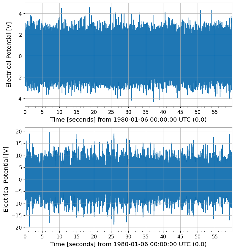
# --- Wrap the drive and response as TimeSeries so the same workflow applies to experimental channels. ---
ts_input = TimeSeries(input_data, t0=0, sample_rate=fs, name="Input", unit="V")
ts_output = TimeSeries(output_data, t0=0, sample_rate=fs, name="Output", unit="V")

print("Input data shape:", ts_input.shape)
print("Output data shape:", ts_output.shape)
Plot(ts_input, ts_output, separate=True);

Input data shape: (122880,)
Output data shape: (122880,)

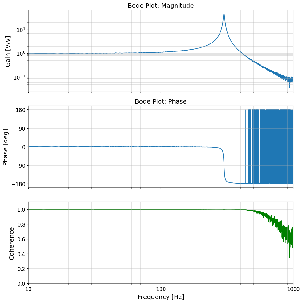
2. Transfer Function Estimation

From the input-output time series data ts_input and ts_output, we estimate the frequency response function (transfer function). We use the transfer_function method of gwexpy.

We also calculate the coherence to assess the reliability of the measurement. Frequency bands where the coherence is close to 1 indicate that the input-output relationship is linear and the influence of noise is small.

# FFT settings: average 2-second segments so random measurement noise is reduced without washing out the 300 Hz resonance.
fftlength = 2.0  # FFT every 2 seconds and average

# Estimate Output/Input so the plant response appears directly in gain and phase.
tf = ts_input.transfer_function(ts_output, fftlength=fftlength)

# Coherence is the confidence check: low coherence means the response is noise dominated and the transfer estimate should not be over-interpreted.
coh = ts_input.coherence(ts_output, fftlength=fftlength) ** 0.5

# --- Plot Bode magnitude, phase, and coherence together so trustworthiness and fitted physics can be read on the same axis. ---
fig, axes = plt.subplots(3, 1, figsize=(10, 10), sharex=True)

# Magnitude
ax = axes[0]
ax.loglog(tf.abs(), label="Measured TF")
ax.set_ylabel("Gain [V/V]")
ax.set_title("Bode Plot: Magnitude")
ax.grid(True, which="both", alpha=0.5)

# Phase
ax = axes[1]
ax.plot(tf.degree(), label="Measured Phase")
ax.set_ylabel("Phase [deg]")
ax.set_title("Bode Plot: Phase")
ax.set_yticks(np.arange(-180, 181, 90))
ax.grid(True, which="both", alpha=0.5)

# Coherence
ax = axes[2]
ax.plot(coh, color="green", label="Coherence")
ax.set_ylabel("Coherence")
ax.set_xlabel("Frequency [Hz]")
ax.set_ylim(0, 1.1)
ax.set_xlim(10, 1000)
ax.grid(True, which="both", alpha=0.5)

plt.tight_layout()
plt.show()

3. Model Fitting

We fit a theoretical model to the obtained transfer function (especially around the resonance). Here, we define a transfer function model for a harmonic oscillator and use least-squares fitting to determine the parameters (\(A, f_0, Q\)).

Model equation (including gain \(A\)):

\[H(f) = A \cdot \frac{f_0^2}{f_0^2 - f^2 + i (f f_0 / Q)}\]

# --- Define a resonator model whose parameters map back to measurable plant physics. ---
def resonator_model(f, amp, f0, Q):
    # f: frequency array in Hz where the measured plant response is sampled.
    # amp scales the actuator/sensor gain, f0 is the modal resonance, and Q controls how sharply energy stays trapped near that mode.

    # Use the complex response so the fit respects both magnitude and phase, not just the height of the peak.
    numerator = amp * (f0**2)
    denominator = (f0**2) - (f**2) + 1j * (f * f0 / Q)
    return numerator / denominator


# --- Fit only the resonance-dominated band so broadband tails do not bias the modal parameters. ---
# Fitting the full band would force one second-order model to explain off-resonance structure it was never meant to capture,
# so we isolate 100-500 Hz where the identified mode dominates the response.
tf_crop = tf.crop(100, 500)

# Seed f0 near the visible peak so the optimizer lands on the physical resonance instead of a spurious local minimum.
# The initial guess is intentionally close to the observed resonance around 300 Hz.
p0 = {"amp": 1.0, "f0": 300.0, "Q": 10.0}

# Fit the complex transfer function in this narrowed band.
# .fit() uses both real and imaginary parts, which preserves phase information needed to recover damping consistently.
result = tf_crop.fit(resonator_model, p0=p0)

print(result)

┌─────────────────────────────────────────────────────────────────────────┐
│                                Migrad                                   │
├──────────────────────────────────┬──────────────────────────────────────┤
│ FCN = 5.83 (χ²/ndof = 0.0)       │              Nfcn = 118              │
│ EDM = 4.62e-06 (Goal: 0.0002)    │                                      │
├──────────────────────────────────┼──────────────────────────────────────┤
│          Valid Minimum           │   Below EDM threshold (goal x 10)    │
├──────────────────────────────────┼──────────────────────────────────────┤
│      No parameters at limit      │           Below call limit           │
├──────────────────────────────────┼──────────────────────────────────────┤
│             Hesse ok             │         Covariance accurate          │
└──────────────────────────────────┴──────────────────────────────────────┘
┌───┬──────┬───────────┬───────────┬────────────┬────────────┬─────────┬─────────┬───────┐
│   │ Name │   Value   │ Hesse Err │ Minos Err- │ Minos Err+ │ Limit-  │ Limit+  │ Fixed │
├───┼──────┼───────────┼───────────┼────────────┼────────────┼─────────┼─────────┼───────┤
│ 0 │ amp  │   0.934   │   0.007   │            │            │         │         │       │
│ 1 │ f0   │  299.997  │   0.021   │            │            │         │         │       │
│ 2 │ Q    │   49.4    │    0.5    │            │            │         │         │       │
└───┴──────┴───────────┴───────────┴────────────┴────────────┴─────────┴─────────┴───────┘
┌─────┬────────────────────────────┐
│     │      amp       f0        Q │
├─────┼────────────────────────────┤
│ amp │ 4.34e-05       -0 -2.29e-3 │
│  f0 │       -0 0.000454  -0.1e-3 │
│   Q │ -2.29e-3  -0.1e-3    0.241 │
└─────┴────────────────────────────┘

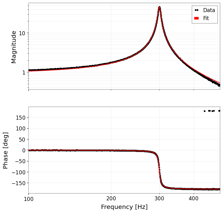
4. Verification of Results

We verify the fitting results numerically and plot them overlaid on the measured data. The FitResult.plot() method automatically generates a Bode plot (magnitude and phase) for complex data.

# --- Report the recovered modal parameters so they can be compared with the known plant values. ---
print("--- Estimated Parameters ---")
print(f"Resonance Frequency (f0): {result.params['f0']:.4f} Hz (True: {f0_true})")
print(f"Quality Factor (Q):       {result.params['Q']:.4f}      (True: {Q_true})")
print(f"Gain (Amp):               {result.params['amp']:.4f}")

# --- Plot the fitted response to confirm that both the peak height and phase rotation are captured. ---
# result.plot() returns magnitude and phase axes because both observables are needed to judge whether the modal model is credible.
axes = result.plot()
plt.show()

--- Estimated Parameters ---
Resonance Frequency (f0): 299.9968 Hz (True: 300.0)
Quality Factor (Q):       49.4100      (True: 50.0)
Gain (Amp):               0.9343