Note

このページは Jupyter Notebook から生成されました。 ノートブックをダウンロード (.ipynb)

# Skipped in CI: Colab/bootstrap dependency install cell.

ケーススタディのフロー:

• メインのギャラリーに戻る: ケーススタディ一覧

• 関連リファレンス: リファレンス総合入口, API: 周波数系列, トピック別参照

• 前後の注目ワークフロー: ノイズバジェット解析, アクティブダンピング

チュートリアル: 伝達関数の測定

このチュートリアルでは、gwexpy を使用して測定データからシステムの伝達関数（Transfer Function）を推定し、 物理モデルへのフィッティングを行ってパラメータを同定する流れを解説します。

シナリオ: ある機械振動系（または電気回路）に白色雑音を入力し、その応答を測定しました。 この入出力データから、システムの共振周波数 \(f_0\) と Q値 \(Q\) を求めます。

ワークフロー:

1. データ生成: 入力信号（白色雑音）と、それに対するシステムの出力（共振系応答 + 測定ノイズ）をシミュレーションします。

2. 伝達関数の推定: 入出力の時系列データから伝達関数とコヒーレンスを計算し、ボード線図（Bode Plot）を描画します。

3. モデルフィッティング: 推定した伝達関数に理論モデル（ローレンツ関数など）を当てはめ、パラメータを推定します。

import warnings

warnings.filterwarnings("ignore", category=UserWarning)
warnings.filterwarnings("ignore", category=DeprecationWarning)

import matplotlib.pyplot as plt
import numpy as np
from scipy import signal

from gwexpy import TimeSeries
from gwexpy.plot import Plot

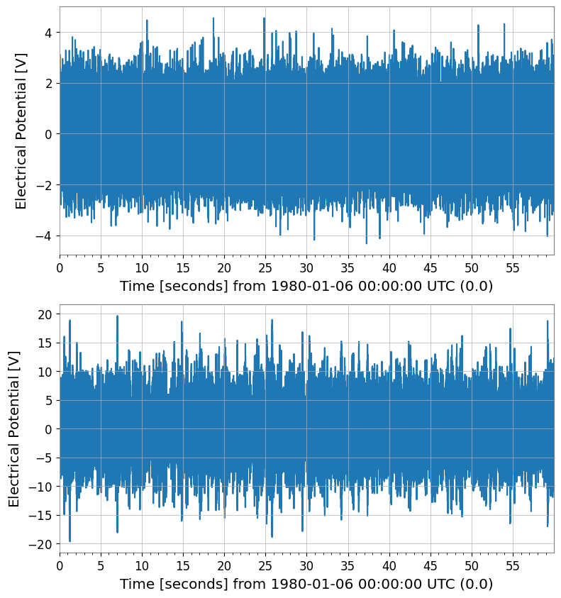
1. 実験データの生成（シミュレーション）

仮想的な実験を行います。

• システム: 2次共振系（単振動）

  • 共振周波数 \(f_0 = 300\) Hz

  • Q値 \(Q = 50\)

• 入力: 白色雑音（White Noise）

• 測定: サンプリング周波数 2048 Hz, 継続時間 60秒

出力信号には、測定に伴うノイズも付加します。

# --- Parameter Settings: choose a resonator whose f0 and Q mimic a narrow mechanical mode worth identifying from measured data. ---
fs = 2048.0  # Sampling frequency [Hz]
duration = 60.0  # Duration [s]
f0_true = 300.0  # True resonance frequency [Hz]
Q_true = 50.0  # True quality factor

# --- Time axis and input signal: broadband drive excites the plant across frequency so the resonance can be measured in one experiment. ---
t = np.linspace(0, duration, int(duration * fs), endpoint=False)
input_data = np.random.normal(0, 1, size=len(t))  # Broadband excitation approximates a swept identification drive without privileging one frequency.

# --- Physical System Simulation (using scipy.signal): this second-order plant stands in for a suspension or actuator resonance. ---
# H(s) uses f0 for the modal frequency and Q for damping width, so fitting them back out tests whether the measurement preserves the true mode shape.
w0 = 2 * np.pi * f0_true
num = [w0**2]
den = [1, w0 / Q_true, w0**2]
system = signal.TransferFunction(num, den)

# Simulate the time response to the broadband drive so transfer estimation sees the same finite-duration effects as a real measurement.
_, output_clean, _ = signal.lsim(system, U=input_data, T=t)

# --- Add measurement noise: coherence later tells us whether this readout noise is low enough to trust the estimated transfer function. ---
# Treat this as sensor/readout noise, which degrades phase and gain estimates where the plant response is weak.
measurement_noise = np.random.normal(0, 0.1, size=len(t))
output_data = output_clean + measurement_noise

# --- Wrap the drive and response as TimeSeries so the same workflow applies to experimental channels. ---
ts_input = TimeSeries(input_data, t0=0, sample_rate=fs, name="Input", unit="V")
ts_output = TimeSeries(output_data, t0=0, sample_rate=fs, name="Output", unit="V")

print("Input data shape:", ts_input.shape)
print("Output data shape:", ts_output.shape)
Plot(ts_input, ts_output, separate=True);

Input data shape: (122880,)
Output data shape: (122880,)

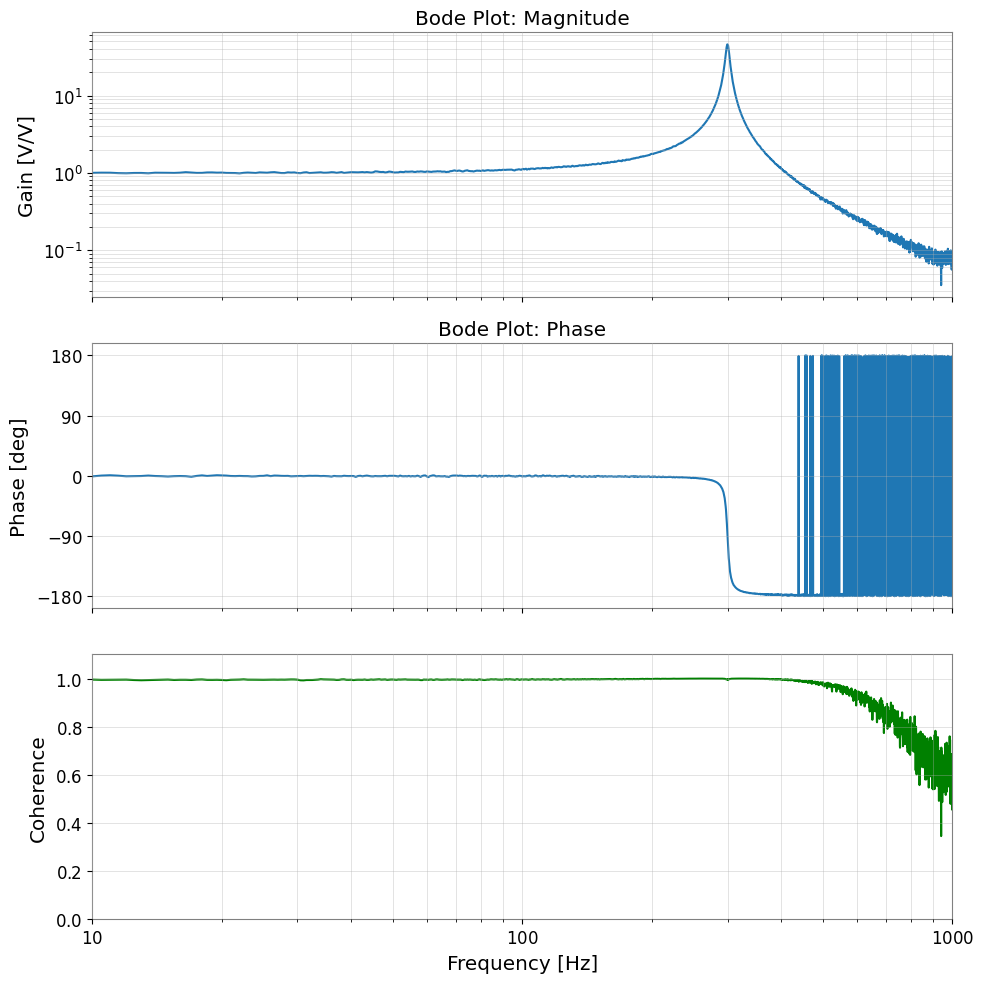
2. 伝達関数の推定

入出力の時系列データ ts_input と ts_output から、周波数応答関数（伝達関数）を推定します。 gwexpy の transfer_function メソッドを使用します。

また、測定の信頼性を確認するためにコヒーレンス（Coherence）も計算します。 コヒーレンスが 1 に近い周波数帯域は、入出力の関係が線形であり、ノイズの影響が少ないことを示します。

# FFT settings: average 2-second segments so random measurement noise is reduced without washing out the 300 Hz resonance.
fftlength = 2.0  # FFT every 2 seconds and average

# Estimate Output/Input so the plant response appears directly in gain and phase.
tf = ts_input.transfer_function(ts_output, fftlength=fftlength)

# Coherence is the confidence check: low coherence means the response is noise dominated and the transfer estimate should not be over-interpreted.
coh = ts_input.coherence(ts_output, fftlength=fftlength) ** 0.5

# --- Plot Bode magnitude, phase, and coherence together so trustworthiness and fitted physics can be read on the same axis. ---
fig, axes = plt.subplots(3, 1, figsize=(10, 10), sharex=True)

# Magnitude
ax = axes[0]
ax.loglog(tf.abs(), label="Measured TF")
ax.set_ylabel("Gain [V/V]")
ax.set_title("Bode Plot: Magnitude")
ax.grid(True, which="both", alpha=0.5)

# Phase
ax = axes[1]
ax.plot(tf.degree(), label="Measured Phase")
ax.set_ylabel("Phase [deg]")
ax.set_title("Bode Plot: Phase")
ax.set_yticks(np.arange(-180, 181, 90))
ax.grid(True, which="both", alpha=0.5)

# Coherence
ax = axes[2]
ax.plot(coh, color="green", label="Coherence")
ax.set_ylabel("Coherence")
ax.set_xlabel("Frequency [Hz]")
ax.set_ylim(0, 1.1)
ax.set_xlim(10, 1000)
ax.grid(True, which="both", alpha=0.5)

plt.tight_layout()
plt.show()

3. モデルフィッティング

得られた伝達関数（特に共振付近）に対して、理論モデルをフィッティングします。 ここでは、単振動の伝達関数モデルを定義し、最小二乗法でパラメータ（\(A, f_0, Q\)）を求めます。

モデル式（ゲイン \(A\) を含む）:

\[H(f) = A \cdot \frac{f_0^2}{f_0^2 - f^2 + i (f f_0 / Q)}\]

# --- Define a resonator model whose parameters map back to measurable plant physics. ---
def resonator_model(f, amp, f0, Q):
    # f: frequency array in Hz where the measured plant response is sampled.
    # amp scales the actuator/sensor gain, f0 is the modal resonance, and Q controls how sharply energy stays trapped near that mode.

    # Use the complex response so the fit respects both magnitude and phase, not just the height of the peak.
    numerator = amp * (f0**2)
    denominator = (f0**2) - (f**2) + 1j * (f * f0 / Q)
    return numerator / denominator


# --- Fit only the resonance-dominated band so broadband tails do not bias the modal parameters. ---
# Fitting the full band would force one second-order model to explain off-resonance structure it was never meant to capture,
# so we isolate 100-500 Hz where the identified mode dominates the response.
tf_crop = tf.crop(100, 500)

# Seed f0 near the visible peak so the optimizer lands on the physical resonance instead of a spurious local minimum.
# The initial guess is intentionally close to the observed resonance around 300 Hz.
p0 = {"amp": 1.0, "f0": 300.0, "Q": 10.0}

# Fit the complex transfer function in this narrowed band.
# .fit() uses both real and imaginary parts, which preserves phase information needed to recover damping consistently.
result = tf_crop.fit(resonator_model, p0=p0)

print(result)

┌─────────────────────────────────────────────────────────────────────────┐
│                                Migrad                                   │
├──────────────────────────────────┬──────────────────────────────────────┤
│ FCN = 5.83 (χ²/ndof = 0.0)       │              Nfcn = 118              │
│ EDM = 4.62e-06 (Goal: 0.0002)    │                                      │
├──────────────────────────────────┼──────────────────────────────────────┤
│          Valid Minimum           │   Below EDM threshold (goal x 10)    │
├──────────────────────────────────┼──────────────────────────────────────┤
│      No parameters at limit      │           Below call limit           │
├──────────────────────────────────┼──────────────────────────────────────┤
│             Hesse ok             │         Covariance accurate          │
└──────────────────────────────────┴──────────────────────────────────────┘
┌───┬──────┬───────────┬───────────┬────────────┬────────────┬─────────┬─────────┬───────┐
│   │ Name │   Value   │ Hesse Err │ Minos Err- │ Minos Err+ │ Limit-  │ Limit+  │ Fixed │
├───┼──────┼───────────┼───────────┼────────────┼────────────┼─────────┼─────────┼───────┤
│ 0 │ amp  │   0.934   │   0.007   │            │            │         │         │       │
│ 1 │ f0   │  299.997  │   0.021   │            │            │         │         │       │
│ 2 │ Q    │   49.4    │    0.5    │            │            │         │         │       │
└───┴──────┴───────────┴───────────┴────────────┴────────────┴─────────┴─────────┴───────┘
┌─────┬────────────────────────────┐
│     │      amp       f0        Q │
├─────┼────────────────────────────┤
│ amp │ 4.34e-05       -0 -2.29e-3 │
│  f0 │       -0 0.000454  -0.1e-3 │
│   Q │ -2.29e-3  -0.1e-3    0.241 │
└─────┴────────────────────────────┘

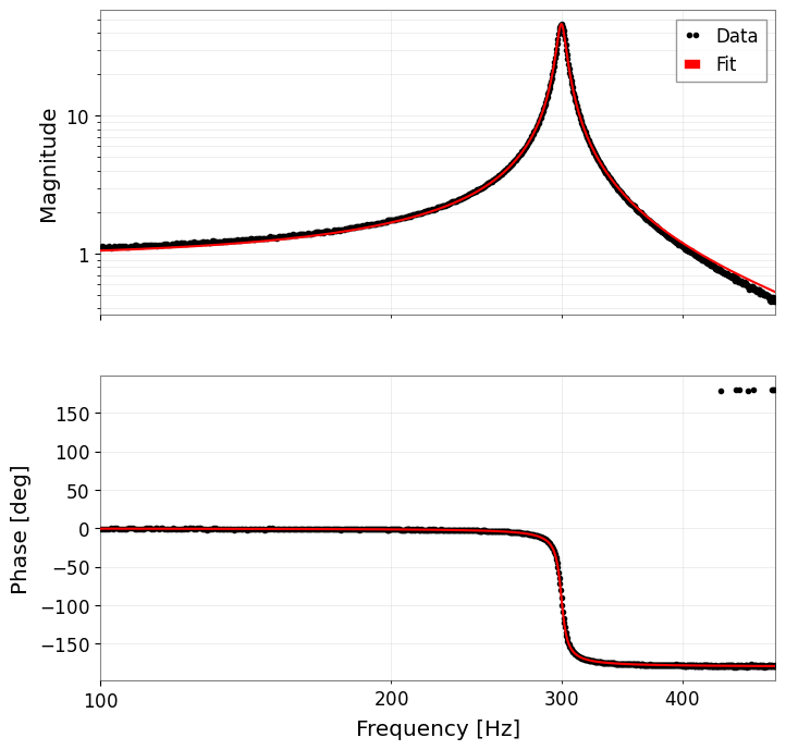
4. 結果の確認

フィッティング結果を数値で確認し、測定データに重ねてプロットします。 FitResult.plot() メソッドは、複素数データの場合、自動的にボード線図（振幅・位相）を描画します。

# --- Report the recovered modal parameters so they can be compared with the known plant values. ---
print("--- Estimated Parameters ---")
print(f"Resonance Frequency (f0): {result.params['f0']:.4f} Hz (True: {f0_true})")
print(f"Quality Factor (Q):       {result.params['Q']:.4f}      (True: {Q_true})")
print(f"Gain (Amp):               {result.params['amp']:.4f}")

# --- Plot the fitted response to confirm that both the peak height and phase rotation are captured. ---
# result.plot() returns magnitude and phase axes because both observables are needed to judge whether the modal model is credible.
axes = result.plot()
plt.show()

--- Estimated Parameters ---
Resonance Frequency (f0): 299.9968 Hz (True: 300.0)
Quality Factor (Q):       49.4100      (True: 50.0)
Gain (Amp):               0.9343