Note
このページは Jupyter Notebook から生成されました。 ノートブックをダウンロード (.ipynb)
[1]:
# Skipped in CI: Colab/bootstrap dependency install cell.
分解解析: PCA・ICA と固有モード
![]()
このチュートリアルでは TimeSeriesMatrix を使った 主成分分析(PCA) と 独立成分分析(ICA) を解説します。
どちらも tsm.pca() / tsm.ica() という高レベル API として利用可能で、内部では scikit-learn をラップしています。
代表的なユースケース:
PCA: 次元削減、相関センサーチャンネルの非相関化
ICA: 盲目信号分離(BSS)— 環境ノイズから物理信号を分離する
sklearn.decomposition.PCA / FastICA を直接使っていたコードは matrix.pca() / matrix.ica() に置き換えられます。[2]:
import warnings

warnings.filterwarnings("ignore", category=UserWarning)
warnings.filterwarnings("ignore", category=DeprecationWarning)

import matplotlib.pyplot as plt
import numpy as np
from astropy import units as u

from gwexpy.timeseries import TimeSeriesMatrix
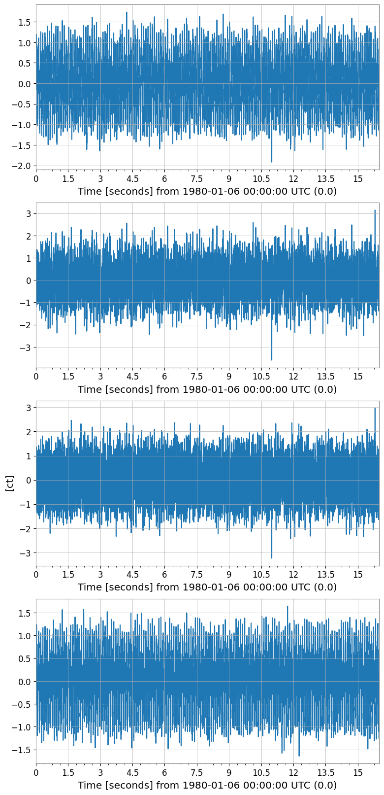
1. マルチチャンネル合成データの準備
現実的なシナリオを再現します:
隠れた信号源 2本: 10 Hz サイン波とブロードバンドノイズ
観測チャンネル 4本: 信号源の線形混合
これは重力波検出器で複数のセンサーに物理信号が混合して現れる状況を模倣しています。
[3]:
rng = np.random.default_rng(42)

fs = 512      # sample rate [Hz]
T  = 16.0     # duration [s]
n  = int(fs * T)
t  = np.arange(n) / fs

# Two independent source signals
src1 = np.sin(2 * np.pi * 10.0 * t)                   # 10 Hz tone
src2 = rng.normal(0, 1, n)                              # broadband noise
src3 = np.sin(2 * np.pi * 40.0 * t + 0.7)             # 40 Hz tone

# Mixing matrix (4 observed channels from 3 sources)
A = np.array([
    [0.8,  0.3,  0.1],
    [0.4,  0.7,  0.2],
    [0.2,  0.5,  0.9],
    [0.6, -0.2,  0.5],
])

sources = np.stack([src1, src2, src3], axis=0)   # (3, n)
mixed   = A @ sources                             # (4, n)

# Add small instrument noise
mixed += 0.05 * rng.normal(0, 1, mixed.shape)

# Build TimeSeriesMatrix (4 channels × 1 col × n samples)
dt = (1 / fs) * u.s
t0 = 0 * u.s

data_3d = mixed[:, np.newaxis, :]   # (4, 1, n)

tsm = TimeSeriesMatrix(
    data_3d,
    dt=dt,
    t0=t0,
    units=np.full((4, 1), u.ct),
)
tsm.channel_names = [f"CH{i}" for i in range(4)]

print("TimeSeriesMatrix shape:", tsm.shape)   # (4, 1, 8192)
tsm.plot(subplots=True, xscale="seconds");
TimeSeriesMatrix shape: (4, 1, 8192)
2. PCA – 次元削減
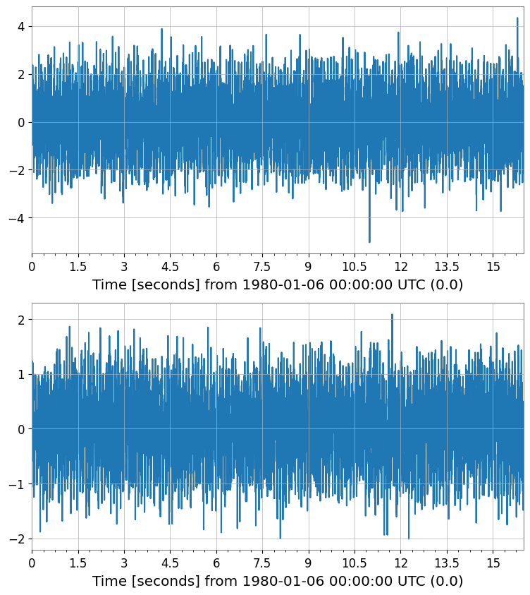
TimeSeriesMatrix.pca() はスコア行列と、オプションで PCAResult オブジェクトを返します。
[4]:
# Fit PCA – keep 2 principal components out of 4 channels
pca_scores, pca_res = tsm.pca(n_components=2, return_model=True)

print("PCA score shape:", pca_scores.shape)           # (2, 1, n)
print("Explained variance ratio:", pca_res.explained_variance_ratio)

pca_scores.plot(subplots=True, xscale="seconds");
PCA score shape: (2, 1, 8192)
Explained variance ratio: [0.68552389 0.18734173]
[5]:
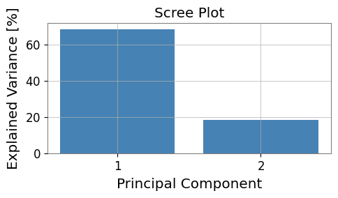
# Visualize explained variance (scree plot)
fig, ax = plt.subplots(figsize=(5, 3))

evr = pca_res.explained_variance_ratio
ax.bar(range(1, len(evr) + 1), evr * 100, color="steelblue")
ax.set_xlabel("Principal Component")
ax.set_ylabel("Explained Variance [%]")
ax.set_title("Scree Plot")
ax.set_xticks(range(1, len(evr) + 1))
plt.tight_layout()
[6]:
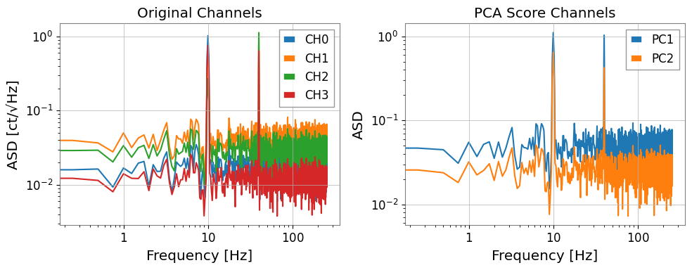
# Compare ASD of original channels vs PC scores
fig, axes = plt.subplots(1, 2, figsize=(10, 4))

asd_orig = tsm.asd(fftlength=4, overlap=0.5)
for i in range(asd_orig.shape[0]):
    axes[0].loglog(
        asd_orig[i, 0].frequencies.value,
        asd_orig[i, 0].value,
        label=f"CH{i}",
    )
axes[0].set_xlabel("Frequency [Hz]")
axes[0].set_ylabel("ASD [ct/√Hz]")
axes[0].set_title("Original Channels")
axes[0].legend()

asd_pca = pca_scores.asd(fftlength=4, overlap=0.5)
for i in range(asd_pca.shape[0]):
    axes[1].loglog(
        asd_pca[i, 0].frequencies.value,
        asd_pca[i, 0].value,
        label=f"PC{i+1}",
    )
axes[1].set_xlabel("Frequency [Hz]")
axes[1].set_ylabel("ASD")
axes[1].set_title("PCA Score Channels")
axes[1].legend()

plt.tight_layout()
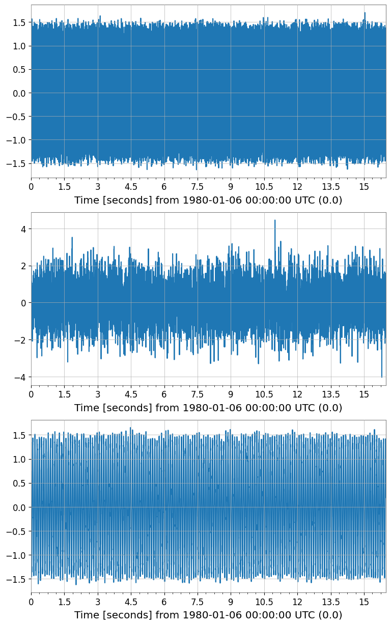
3. ICA – 盲目信号分離
TimeSeriesMatrix.ica() は FastICA を実行し、独立成分行列を返します。
[7]:
# Fit ICA – recover 3 independent components
ica_sources = tsm.ica(n_components=3, random_state=0)

print("ICA source shape:", ica_sources.shape)   # (3, 1, n)

ica_sources.plot(subplots=True, xscale="seconds");
ICA source shape: (3, 1, 8192)
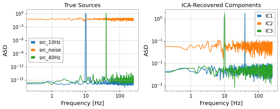
[8]:
# Compare ICA sources vs. known sources in frequency domain
fig, axes = plt.subplots(1, 2, figsize=(10, 4))

# True sources (for reference)
src_3d = np.stack([src1, src2, src3], axis=0)[:, np.newaxis, :]  # (3,1,n)
tsm_src = TimeSeriesMatrix(src_3d, dt=dt, t0=t0)
tsm_src.channel_names = ["src_10Hz", "src_noise", "src_40Hz"]
asd_src = tsm_src.asd(fftlength=4, overlap=0.5)

for i in range(3):
    axes[0].loglog(
        asd_src[i, 0].frequencies.value,
        asd_src[i, 0].value,
        label=tsm_src.channel_names[i],
    )
axes[0].set_title("True Sources")
axes[0].set_xlabel("Frequency [Hz]")
axes[0].set_ylabel("ASD")
axes[0].legend()

asd_ica = ica_sources.asd(fftlength=4, overlap=0.5)
for i in range(asd_ica.shape[0]):
    axes[1].loglog(
        asd_ica[i, 0].frequencies.value,
        asd_ica[i, 0].value,
        label=f"IC{i+1}",
    )
axes[1].set_title("ICA-Recovered Components")
axes[1].set_xlabel("Frequency [Hz]")
axes[1].set_ylabel("ASD")
axes[1].legend()

plt.tight_layout()
4. 前処理:標準化とホワイトニング
ICA・PCA にはスケーリングが重要です。TimeSeriesMatrix には組み込み前処理が備わっています:
メソッド |
説明 |
|---|---|
|
各チャンネルを平均 0、分散 1 に正規化 |
|
外れ値に強い中央値/MAD スケーリング |
|
PCA ホワイトニング(チャンネル間相関の除去) |
pca() / ica() には scale パラメータで内部適用も可能です。
[9]:
# Manual preprocessing pipeline
tsm_z = tsm.standardize(method='zscore')

print("Mean  ≈ 0:", np.allclose(tsm_z.value.mean(axis=-1), 0, atol=1e-10))
print("Std   ≈ 1:", np.allclose(tsm_z.value.std(axis=-1),  1, atol=0.01))

# ICA with internal z-score scaling
ica_scaled = tsm.ica(n_components=3, scale='zscore', random_state=0)
print("ICA (with zscore) shape:", ica_scaled.shape)

# PCA with robust scaling
pca_robust, pca_res2 = tsm.pca(n_components=2, scale='robust', return_model=True)
print("PCA (robust) EVR:", pca_res2.explained_variance_ratio)
Mean  ≈ 0: True
Std   ≈ 1: True
ICA (with zscore) shape: (3, 1, 8192)
PCA (robust) EVR: [0.44248267 0.37626797]
5. 欠損値 (NaN) の取り扱い
実際のデータには観測ギャップがある場合があります。nan_policy='impute' で分解前に補完できます。
[10]:
# Inject some NaN gaps (simulating data gaps)
tsm_nan = tsm.copy()
tsm_nan.value[0, 0, 100:120] = np.nan
tsm_nan.value[2, 0, 500:510] = np.nan

print("NaN count:", np.sum(np.isnan(tsm_nan.value)))

# PCA with linear interpolation of NaN gaps
pca_nanfill, _ = tsm_nan.pca(
    n_components=2,
    nan_policy='impute',
    impute_kwargs={'method': 'interpolate'},
    return_model=True,
)
print("PCA (nan impute) shape:", pca_nanfill.shape)
NaN count: 30
PCA (nan impute) shape: (2, 1, 8192)
6. scikit-learn からの移行ガイド
移行前(scikit-learn 直接使用):
from sklearn.decomposition import PCA, FastICA
import numpy as np

# 生の numpy 配列 (n_samples, n_channels)
X = data.reshape(n_channels, n_samples).T

pca = PCA(n_components=2)
scores = pca.fit_transform(X)           # (n_samples, 2)

ica = FastICA(n_components=3, random_state=0)
sources = ica.fit_transform(X)          # (n_samples, 3)
移行後(gwexpy):
# dt/t0/unit を保持したまま処理
pca_scores, pca_res = tsm.pca(n_components=2, return_model=True)
ica_sources          = tsm.ica(n_components=3, random_state=0)
gwexpy API が自動で行うこと:
時間軸(
dt、t0、times)を出力行列に引き継ぎ単位メタデータを保持
.plot()で直接プロット可能NaN 処理・スケーリングを内部で処理
まとめ
メソッド |
主要パラメータ |
返り値 |
|---|---|---|
|
|
|
|
|
|
どちらのメソッドも TimeSeriesMatrix を返すので、.plot(), .asd(), .coherence() などの後続操作がそのまま使えます。
関連チュートリアル: