Note

このページは Jupyter Notebook から生成されました。 ノートブックをダウンロード (.ipynb)

# Skipped in CI: Colab/bootstrap dependency install cell.

フィッティング: スペクトル線解析

このノートブックでは、gwexpy.fitting モジュールを使用して、TimeSeries や FrequencySeries データに対して簡単にフィッティングを行う方法を紹介します。 バックエンドには iminuit を使用しており、誤差を考慮した最小二乗法フィッティングが可能です。

import warnings

warnings.filterwarnings("ignore", category=UserWarning)
warnings.filterwarnings("ignore", category=DeprecationWarning)

import matplotlib.pyplot as plt
import numpy as np

from gwexpy.frequencyseries import FrequencySeries
from gwexpy.plot import Plot
from gwexpy.timeseries import TimeSeries

plt.rcParams["figure.figsize"] = (10, 6)

1. データの準備

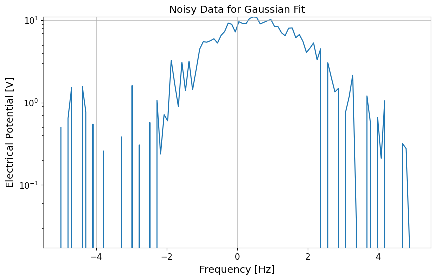
ここでは、ガウス関数にノイズを加えたダミーデータを作成します。

# Define model function (Gaussian)
def gaussian(x, a, mu, sigma):
    return a * np.exp(-((x - mu) ** 2) / (2 * sigma**2))


# Generate dummy data on an explicit x-axis
np.random.seed(42)
x = np.linspace(-5, 5, 100)
true_params = {"a": 10, "mu": 0.5, "sigma": 1.2}
y_true = gaussian(x, **true_params)
y_noise = y_true + np.random.normal(0, 1.0, size=len(x))

# Use FrequencySeries so the fit axis matches the synthetic x values
ts = FrequencySeries(y_noise, frequencies=x, name="Noisy Gaussian", unit="V")
ts.plot(title="Noisy Data for Gaussian Fit");

2. フィッティングの実行

ts.fit() メソッドを使用してフィッティングを行います。 引数にはモデル関数と、パラメータの初期値 p0 を指定します。

狭いピークや局在したピークでは、中心周波数と幅に物理的に妥当な範囲を与え、ノイズだけの局所解へ流れないようにします。

# Fitting
# Keep the initial center near the visible peak and bound (mu, sigma) to plausible values
gaussian_limits = {"mu": (-2.0, 2.0), "sigma": (0.2, 3.0)}
result = ts.fit(
    gaussian,
    sigma=0.8,
    p0={"a": 8.0, "mu": 0.0, "sigma": 1.0},
    limits=gaussian_limits,
)

# Display results
display(result)

Migrad
FCN = 125.2 (χ²/ndof = 1.3)	Nfcn = 85
EDM = 1e-07 (Goal: 0.0002)
Valid Minimum	Below EDM threshold (goal x 10)
No parameters at limit	Below call limit
Hesse ok	Covariance accurate

	Name	Value	Hesse Error	Minos Error-	Minos Error+	Limit-	Limit+	Fixed
0	a	10.05	0.21
1	mu	0.550	0.029			-2	2
2	sigma	1.171	0.028			0.2	3

	a	mu	sigma
a	0.0461	-0 (-0.005)	-3.5e-3 (-0.569)
mu	-0 (-0.005)	0.000845	0 (0.008)
sigma	-3.5e-3 (-0.569)	0 (0.008)	0.00081

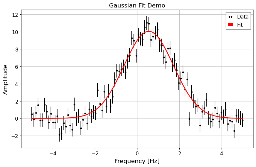
3. 結果の取得とプロット

FitResult オブジェクトから、ベストフィットパラメータや誤差、Chi2 値などを取得できます。 また、.plot() メソッドで簡単に結果を可視化できます。

print("Best Fit Parameters:", result.params)
print("Errors:", result.errors)
print("Chi2:", result.chi2)
print("NDOF:", result.ndof)

# Plot
fig, ax = plt.subplots(figsize=(10, 6))
result.plot(ax=ax, color="red", linewidth=2)
ax.set_title("Gaussian Fit Demo")
# When using auto-gps, let GWpy handle xlabel (includes epoch)
ax.set_ylabel("Amplitude")
plt.show()

Best Fit Parameters: {'a': 10.053068004204636, 'mu': 0.5500233455726176, 'sigma': 1.1710489113863423}
Errors: {'a': 0.21465081142898548, 'mu': 0.029072612232381, 'sigma': 0.02846288328581481}
Chi2: 125.15392534185452
NDOF: 97

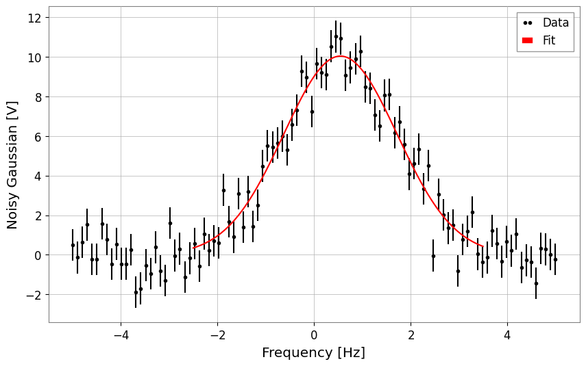
3. 文字列によるモデル指定

モデル関数を定義する代わりに、定義済みのモデル名を文字列で指定することもできます。 現在サポートされているモデル: 'gaus', 'exp', 'pol0', 'pol1', … 'pol9', 'landau' など。

以下は 'gaus' を指定してフィッティングを行う例です。こちらも、目に見えているピーク帯域だけを切り出して callable 版と同じ問題設定に揃えます。

# Fit using string 'gaus'
# Note: Parameter names for predefined models are fixed (for Gaussian: A, mu, sigma)
result_str = ts.fit(
    "gaus",
    p0={"A": 8.0, "mu": 0.0, "sigma": 1.0},
    x_range=(-2.5, 3.5),
    sigma=0.8,
    limits={"mu": (-2.0, 2.0), "sigma": (0.2, 3.0)},
)

# Display results
display(result_str)
result_str.plot();

Migrad
FCN = 81.36 (χ²/ndof = 1.4)	Nfcn = 85
EDM = 1.24e-08 (Goal: 0.0002)
Valid Minimum	Below EDM threshold (goal x 10)
No parameters at limit	Below call limit
Hesse ok	Covariance accurate

	Name	Value	Hesse Error	Minos Error-	Minos Error+	Limit-	Limit+	Fixed
0	A	10.04	0.22
1	mu	0.548	0.029			-2	2
2	sigma	1.175	0.029			0.2	3

	A	mu	sigma
A	0.0466	0 (0.002)	-3.7e-3 (-0.578)
mu	0 (0.002)	0.000854	-0 (-0.003)
sigma	-3.7e-3 (-0.578)	-0 (-0.003)	0.000858

4. 複素数フィッティング (伝達関数)

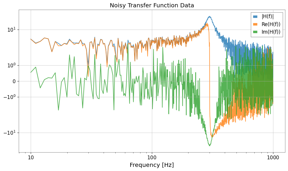
伝達関数などの複素数データに対してもフィッティングを行えます。 コスト関数として \(\chi^2 = \sum (Re_{diff})^2 + \sum (Im_{diff})^2\) を最小化し、実部と虚部を同時にフィットします。 結果のプロットは自動的にボード線図（振幅・位相）になります。

# 1. Define complex model (simple pole)
def pole_model(f, A, f0, Q):
    # H(f) = A / (1 + i * Q * (f/f0 - f0/f))
    # Low-pass filter like but simplified. Let's use standard mechanical transfer function:
    # H(f) = A / [ (f0^2 - f^2) + i * (f0 * f / Q) ]
    omega = 2 * np.pi * f
    omega0 = 2 * np.pi * f0
    return A / ((omega0**2 - omega**2) + 1j * (omega0 * omega / Q))


# 2. Generate data
f = np.linspace(10, 1000, 1000)
p_true = {"A": 1e7, "f0": 300, "Q": 10}
data_clean = pole_model(f, **p_true)

# Add noise (real and imaginary parts independent)
np.random.seed(0)
noise_re = np.random.normal(0, 5, len(f))
noise_im = np.random.normal(0, 5, len(f))
data_noisy = data_clean + 0.2 * noise_re + 0.2j * noise_im

# Create FrequencySeries
fs = FrequencySeries(data_noisy, frequencies=f, name="Transfer Function")
plot = Plot(fs.abs(), fs.real, fs.imag, xscale="log", yscale="symlog", alpha=0.8)
plt.legend(["|H(f)|", "Re(H(f))", "Im(H(f))"])
plt.title("Noisy Transfer Function Data")
plt.tight_layout()
plt.show()

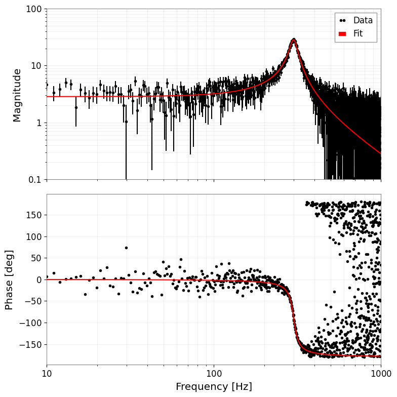
# 3. Fitting
print("Fit Start...")
# Use shifted initial values
result_complex = fs.fit(pole_model, sigma=1.0, p0={"A": 0.8e7, "f0": 320, "Q": 8})

# Display results
display(result_complex)

# 4. Plot (Bode plot)
# Automatically becomes amplitude and phase plots
result_complex.bode_plot()
plt.gcf().get_axes()[0].set_ylim(1e-1, 1e2)
plt.tight_layout()
plt.show()

Fit Start...

Migrad
FCN = 1907 (χ²/ndof = 1.0)	Nfcn = 102
EDM = 1.21e-09 (Goal: 0.0002)
Valid Minimum	Below EDM threshold (goal x 10)
No parameters at limit	Below call limit
Hesse ok	Covariance accurate

	Name	Value	Hesse Error	Minos Error-	Minos Error+	Limit-	Limit+	Fixed
0	A	10.09e6	0.07e6
1	f0	300.24	0.11
2	Q	9.99	0.10

	A	f0	Q
A	5.4e+09	795.222 (0.099)	-5.296459e3 (-0.707)
f0	795.222 (0.099)	0.0118	-0.000 (-0.035)
Q	-5.296459e3 (-0.707)	-0.000 (-0.035)	0.0104

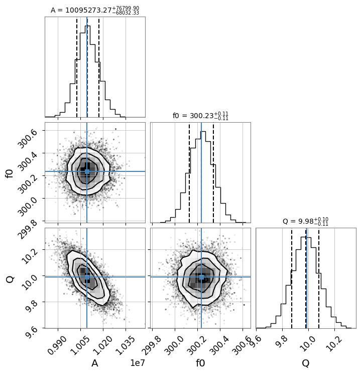
5. MCMC 解析 (emcee)

iminuit で得られた最尤推定値を初期値として、emcee を用いた MCMC (Markov Chain Monte Carlo) 解析を行うことができます。

Note: この機能を使用するには emcee と corner がインストールされている必要があります。

# Run MCMC
# n_walkers: number of walkers, n_steps: number of steps, burn_in: number of initial steps to discard
try:
    sampler = result_complex.run_mcmc(n_walkers=32, n_steps=1000, burn_in=200)

    # Create corner plot (visualize posterior distribution)
    # Display true values (or maximum likelihood estimates) with blue lines
    result_complex.plot_corner()

except ImportError as e:
    print(e)
except Exception as e:
    print(f"MCMC Error: {e}")

100%|██████████| 1000/1000 [00:09<00:00, 102.98it/s]

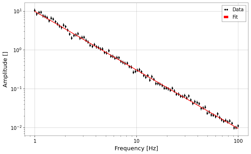
新しい共通モデルの使用例

gwexpy.fitting.models に追加された power_law と damped_oscillation の使用例です。

from gwexpy.fitting.models import damped_oscillation, power_law

# Power law
x = np.logspace(0, 2, 100)
y = power_law(x, A=10, alpha=-1.5) * (1 + 0.1 * np.random.normal(size=len(x)))
fs = FrequencySeries(y, frequencies=x)
res_pl = fs.fit("power_law", p0={"A": 5, "alpha": -1}, sigma=y * 0.1)
print("Power law alpha:", res_pl.params["alpha"])
display(res_pl)
res_pl.plot()
plt.xscale("log")
plt.yscale("log")
plt.show()
plt.close()

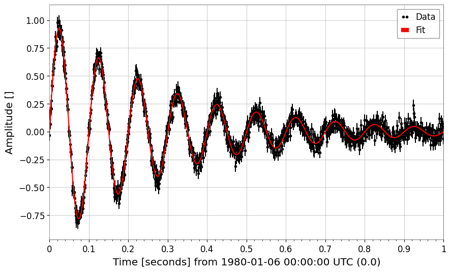
# Damped oscillation
t = np.linspace(0, 1, 1000)
y_osc = damped_oscillation(t, A=1, tau=0.3, f=10) + 0.05 * np.random.normal(size=len(t))
ts_osc = TimeSeries(y_osc, times=t)
res_osc = ts_osc.fit(
    "damped_oscillation", p0={"A": 0.5, "tau": 0.5, "f": 12}, sigma=0.05
)
print("Damped oscillation frequency:", res_osc.params["f"])
display(res_osc)
res_osc.plot();

Power law alpha: -1.507325448901415

Migrad
FCN = 102.8 (χ²/ndof = 1.0)	Nfcn = 90
EDM = 6.45e-06 (Goal: 0.0002)
Valid Minimum	Below EDM threshold (goal x 10)
No parameters at limit	Below call limit
Hesse ok	Covariance accurate

	Name	Value	Hesse Error	Minos Error-	Minos Error+	Limit-	Limit+	Fixed
0	A	9.84	0.20
1	alpha	-1.507	0.008

	A	alpha
A	0.04	-1.33e-3 (-0.869)
alpha	-1.33e-3 (-0.869)	5.88e-05

Damped oscillation frequency: 9.993425925552833

Migrad
FCN = 917.9 (χ²/ndof = 0.9)	Nfcn = 192
EDM = 6.02e-07 (Goal: 0.0002)
Valid Minimum	Below EDM threshold (goal x 10)
No parameters at limit	Below call limit
Hesse ok	Covariance accurate

	Name	Value	Hesse Error	Minos Error-	Minos Error+	Limit-	Limit+	Fixed
0	A	1.002	0.008
1	tau	0.301	0.004
2	f	9.993	0.006
3	phi	0.010	0.008

	A	tau	f	phi
A	6.91e-05	-0.021e-3 (-0.717)	0 (0.072)	-0.01e-3 (-0.104)
tau	-0.021e-3 (-0.717)	1.28e-05	-0.001e-3 (-0.048)	0.002e-3 (0.072)
f	0 (0.072)	-0.001e-3 (-0.048)	3.95e-05	-0.04e-3 (-0.713)
phi	-0.01e-3 (-0.104)	0.002e-3 (0.072)	-0.04e-3 (-0.713)	6.74e-05

7. スペクトル線フィッティング：ローレンツ関数と Voigt プロファイル

重力波検出器のコミッショニングでは、機械共振（バイオリンモード、ペンジュラムモード等）や 注入ライン信号が ASD スペクトル上に鋭いピークとして現れます。

以下の 3 つのプロファイルが広く使われます：

モデル	使いどき
Gaussian	ドップラー・圧力広がり；対称なノイズピーク
Lorentzian	単一損失機構による共振（Q 値で幅が決まる）
Voigt	ガウス（計器分解能）＋ローレンツ（減衰）の複合広がり

いずれも gwexpy.fitting.models に実装済みで、文字列名での指定が可能です。

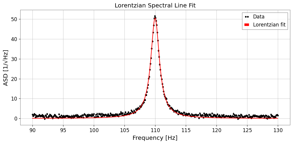
7a. ローレンツ関数（HWHM パラメータ化）

\[f(x) = \frac{A\,\gamma^2}{(x - x_0)^2 + \gamma^2}\]

• A : ピーク振幅

• x0: 中心周波数

• gamma: 半値半幅 (HWHM)

from gwexpy.fitting.models import lorentzian, voigt

# ── Synthetic ASD with a Lorentzian resonance peak ──────────────
np.random.seed(0)
freqs = np.linspace(90, 130, 400)   # Hz, around a 110 Hz mode
TRUE_A, TRUE_X0, TRUE_GAMMA = 50.0, 110.0, 0.8

y_lorenz = lorentzian(freqs, TRUE_A, TRUE_X0, TRUE_GAMMA)
noise = np.random.normal(0, 0.5, len(freqs))
y_data = y_lorenz + noise + 1.0   # +1 flat background

fs_lorenz = FrequencySeries(y_data, frequencies=freqs,
                           name='ASD with Lorentzian peak', unit='1/rtHz')

# ── Fit ─────────────────────────────────────────────────────────
res_lorenz = fs_lorenz.fit(
    'lorentzian',
    p0={'A': 30.0, 'x0': 112.0, 'gamma': 1.5},
    sigma=0.5,
)

print(f"True  A={TRUE_A}, x0={TRUE_X0}, gamma={TRUE_GAMMA}")
print(f"Fit   A={res_lorenz.params['A']:.2f} ± {res_lorenz.errors['A']:.2f}")
print(f"      x0={res_lorenz.params['x0']:.3f} ± {res_lorenz.errors['x0']:.3f}")
print(f"      gamma={res_lorenz.params['gamma']:.3f} ± {res_lorenz.errors['gamma']:.3f}")

fig, ax = plt.subplots(figsize=(10, 5))
res_lorenz.plot(ax=ax, label='Lorentzian fit')
ax.set_xlabel('Frequency [Hz]')
ax.set_ylabel('ASD [1/√Hz]')
ax.set_title('Lorentzian Spectral Line Fit')
ax.legend()
plt.tight_layout()
plt.show()

True  A=50.0, x0=110.0, gamma=0.8
Fit   A=50.50 ± 0.20
      x0=110.000 ± 0.003
      gamma=0.851 ± 0.005

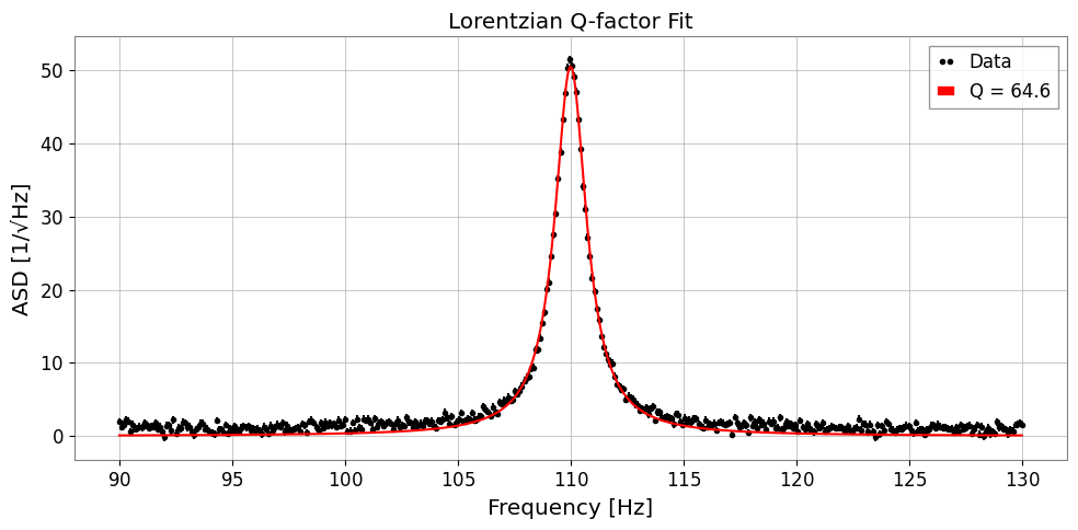
7b. ローレンツ Q 値パラメータ化

共振器では線幅を品質係数 \(Q = x_0 / (2\gamma)\) で表すと直感的です：

\[\gamma = \frac{x_0}{2Q}\]

'lorentzian_q' を使うと (A, x0, Q) を直接フィットできます。

TRUE_Q = TRUE_X0 / (2 * TRUE_GAMMA)   # ~68.75

res_q = fs_lorenz.fit(
    'lorentzian_q',
    p0={'A': 30.0, 'x0': 112.0, 'Q': 50.0},
    sigma=0.5,
)

print(f"True  Q = {TRUE_Q:.2f}")
print(f"Fit   Q = {res_q.params['Q']:.2f} ± {res_q.errors['Q']:.2f}")
print(f"      x0 = {res_q.params['x0']:.3f} ± {res_q.errors['x0']:.3f} Hz")

fig, ax = plt.subplots(figsize=(10, 5))
res_q.plot(ax=ax, label=f"Q = {res_q.params['Q']:.1f}")
ax.set_xlabel('Frequency [Hz]')
ax.set_ylabel('ASD [1/√Hz]')
ax.set_title('Lorentzian Q-factor Fit')
ax.legend()
plt.tight_layout()
plt.show()

True  Q = 68.75
Fit   Q = 64.63 ± 0.36
      x0 = 110.000 ± 0.003 Hz

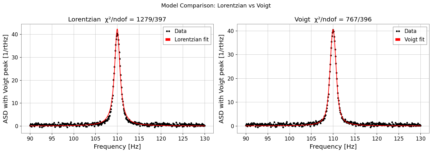
7c. Voigt プロファイル

Voigt プロファイルはガウス関数（幅 \(\sigma\)）とローレンツ関数（HWHM \(\gamma\)）の畳み込みで、 Faddeeva 関数を使って高速計算されます。

計器分解能（ガウス）と内部減衰（ローレンツ）が共存するラインに使用します。

# ── Synthetic data with mixed broadening ─────────────────────────
TRUE_SIGMA, TRUE_GAMMA_V = 0.5, 0.4
y_voigt = voigt(freqs, A=40.0, x0=110.0, sigma=TRUE_SIGMA, gamma=TRUE_GAMMA_V)
y_data_v = y_voigt + np.random.normal(0, 0.4, len(freqs)) + 0.5

fs_voigt = FrequencySeries(y_data_v, frequencies=freqs,
                          name='ASD with Voigt peak', unit='1/rtHz')

# Fit Lorentzian (wrong model) for comparison
res_l = fs_voigt.fit('lorentzian', p0={'A': 30.0, 'x0': 111.0, 'gamma': 0.8},
                     sigma=0.4)

# Fit Voigt (correct model)
res_v = fs_voigt.fit('voigt',
                     p0={'A': 30.0, 'x0': 111.0, 'sigma': 0.6, 'gamma': 0.5},
                     sigma=0.4)

print(f"Lorentzian  chi2/ndof = {res_l.chi2:.1f}/{res_l.ndof}")
print(f"Voigt       chi2/ndof = {res_v.chi2:.1f}/{res_v.ndof}")
print(f"Recovered sigma={res_v.params['sigma']:.3f} (true {TRUE_SIGMA}),"
      f" gamma={res_v.params['gamma']:.3f} (true {TRUE_GAMMA_V})")

fig, axes = plt.subplots(1, 2, figsize=(14, 5))
res_l.plot(ax=axes[0], label='Lorentzian fit')
axes[0].set_title(f"Lorentzian  χ²/ndof = {res_l.chi2:.0f}/{res_l.ndof}")
axes[0].set_xlabel('Frequency [Hz]')
axes[0].legend()

res_v.plot(ax=axes[1], label='Voigt fit')
axes[1].set_title(f"Voigt  χ²/ndof = {res_v.chi2:.0f}/{res_v.ndof}")
axes[1].set_xlabel('Frequency [Hz]')
axes[1].legend()

plt.suptitle('Model Comparison: Lorentzian vs Voigt', fontsize=13)
plt.tight_layout()
plt.show()

Lorentzian  chi2/ndof = 1278.6/397
Voigt       chi2/ndof = 766.8/396
Recovered sigma=0.415 (true 0.5), gamma=0.522 (true 0.4)