Note
このページは Jupyter Notebook から生成されました。 ノートブックをダウンロード (.ipynb)
[1]:
# Skipped in CI: Colab/bootstrap dependency install cell.
カップリング解析: マルチチャンネル結合
![]()
このチュートリアルでは gwexpy.analysis.CouplingFunctionAnalysis を使ったカップリング関数(CF)解析のワークフローを解説します。
カップリング関数とは
カップリング関数は、ウィットネス(環境センサー)のノイズがターゲット(感度チャンネル)にどれだけ結合するかを定量化します:
ここで \(P_{\rm inj}\) と \(P_{\rm bkg}\) はそれぞれ注入時・バックグラウンド時のパワースペクトル密度です。
典型的な用途: KAGRA/LIGO/Virgo の PEM(Physical Environment Monitor)インジェクション解析
注意 — SigmaThreshold の統計的妥当性: 平均化セグメント数
n_avgが 10 未満の場合、χ²(2K) 分布のガウス近似の精度が低下します。この場合UserWarningが発生します。短いデータセグメントではPercentileThresholdの使用を検討してください。
[2]:
import warnings

warnings.filterwarnings("ignore", category=UserWarning)
warnings.filterwarnings("ignore", category=DeprecationWarning)

import matplotlib.pyplot as plt
import numpy as np
from astropy import units as u

from gwexpy.analysis.coupling import (
    CouplingFunctionAnalysis,
    RatioThreshold,
    SigmaThreshold,
)
from gwexpy.timeseries import TimeSeries, TimeSeriesDict
1. 合成インジェクション/バックグラウンドデータの準備
シミュレーション設定:
ウィットネスチャンネル(環境センサー): 地震計・音響センサー
ターゲットチャンネル 2 本: 結合強度の異なる感度計
インジェクションではウィットネスにトーン信号を加えます。ターゲットへの応答は結合強度に比例します。
[3]:
rng = np.random.default_rng(0)

fs   = 512     # sample rate [Hz]
T    = 32.0    # duration [s]
n    = int(fs * T)
t    = np.arange(n) / fs
dt   = (1 / fs) * u.s

# Frequency bins for injected tones
f_inj1 = 12.5   # Hz
f_inj2 = 25.0   # Hz

# Noise floor
noise_level = 0.1

# --- Background data (no injection) ---
wit_bkg  = rng.normal(0, noise_level, n)
tgt1_bkg = rng.normal(0, noise_level, n)
tgt2_bkg = rng.normal(0, noise_level, n)

# --- Injection data: excite the witness with tones ---
inj_signal = 5.0 * np.sin(2 * np.pi * f_inj1 * t) + 3.0 * np.sin(2 * np.pi * f_inj2 * t)

wit_inj  = inj_signal + rng.normal(0, noise_level, n)

# Target 1: strong coupling (CF ≈ 0.4 at f_inj1, 0.3 at f_inj2)
cf_true1 = 0.4
tgt1_inj = cf_true1 * inj_signal + rng.normal(0, noise_level, n)

# Target 2: weak coupling (CF ≈ 0.05)
cf_true2 = 0.05
tgt2_inj = cf_true2 * inj_signal + rng.normal(0, noise_level, n)

# Wrap in TimeSeries
def make_ts(data, name, unit=u.ct):
    return TimeSeries(data, dt=dt, t0=0*u.s, unit=unit, name=name)

# Background dict
data_bkg = TimeSeriesDict({
    "ACC:FLOOR_X":  make_ts(wit_bkg,  "ACC:FLOOR_X",  u.m / u.s**2),
    "GW:DARM":      make_ts(tgt1_bkg, "GW:DARM",      u.m),
    "GW:AUX":       make_ts(tgt2_bkg, "GW:AUX",       u.m),
})

# Injection dict
data_inj = TimeSeriesDict({
    "ACC:FLOOR_X":  make_ts(wit_inj,  "ACC:FLOOR_X",  u.m / u.s**2),
    "GW:DARM":      make_ts(tgt1_inj, "GW:DARM",      u.m),
    "GW:AUX":       make_ts(tgt2_inj, "GW:AUX",       u.m),
})

print("Background channels:", list(data_bkg.keys()))
print("Injection channels: ", list(data_inj.keys()))
Background channels: ['ACC:FLOOR_X', 'GW:DARM', 'GW:AUX']
Injection channels:  ['ACC:FLOOR_X', 'GW:DARM', 'GW:AUX']
2. カップリング関数解析の実行
CouplingFunctionAnalysis.compute() にインジェクション・バックグラウンドの TimeSeriesDict とウィットネスチャンネル名を渡します。
[4]:
cfa = CouplingFunctionAnalysis()

results = cfa.compute(
    data_inj=data_inj,
    data_bkg=data_bkg,
    fftlength=4.0,          # 4-second FFT segments
    overlap=0.5,             # 50% overlap
    witness="ACC:FLOOR_X",  # the environmental sensor
    threshold_witness=RatioThreshold(ratio=10.0),   # witness must show 10× excess
    threshold_target=RatioThreshold(ratio=2.0),     # target must show 2× excess
)

print("Results computed for:", list(results.keys()))
Results computed for: ['GW:DARM', 'GW:AUX']
3. 結果の確認
CouplingResult オブジェクトにカップリング関数・上限・診断 PSD が格納されています。
[5]:
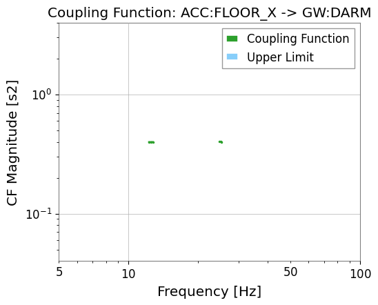
# Strong coupling channel (GW:DARM)
res_darm = results["GW:DARM"]

print("CF valid bins:", res_darm.valid_mask.sum())
print("CF at f_inj1 bin:", end=" ")

freqs = res_darm.cf.frequencies.value
idx1 = np.argmin(np.abs(freqs - f_inj1))
idx2 = np.argmin(np.abs(freqs - f_inj2))
print(f"{res_darm.cf.value[idx1]:.3f} (expected ~{cf_true1})")
print(f"CF at f_inj2 bin: {res_darm.cf.value[idx2]:.3f} (expected ~{cf_true1})")

# Simple CF plot
res_darm.plot_cf(xlim=(5, 100));
CF valid bins: 6
CF at f_inj1 bin: 0.400 (expected ~0.4)
CF at f_inj2 bin: 0.401 (expected ~0.4)
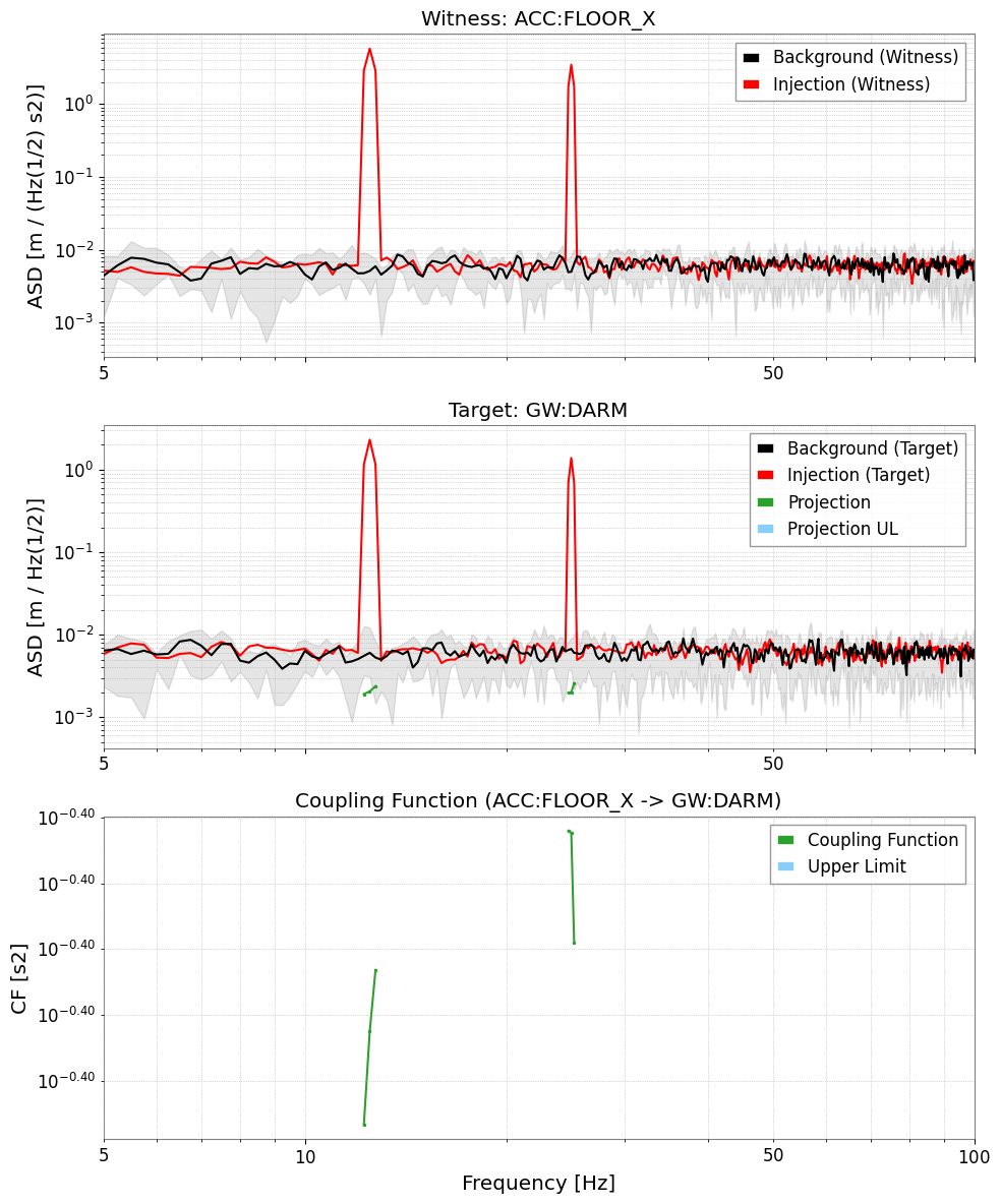
[6]:
# Full diagnostic plot: Witness ASD | Target ASD | CF
res_darm.plot(xlim=(5, 100));
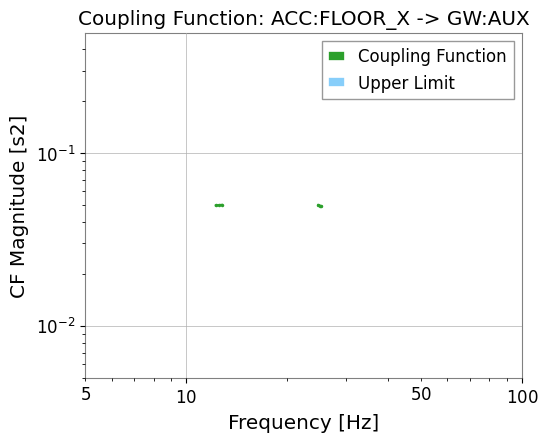
[7]:
# Weak coupling channel (GW:AUX)
res_aux = results["GW:AUX"]
print("GW:AUX valid CF bins:", res_aux.valid_mask.sum())
res_aux.plot_cf(xlim=(5, 100));
GW:AUX valid CF bins: 6
import warnings
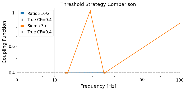
4. 閾値戦略の比較
gwexpy には 3 種類の組み込み閾値戦略があります:
戦略 |
説明 |
適したデータ |
|---|---|---|
|
\(P_{\rm inj} > r \cdot P_{\rm bkg}\) |
高速スクリーニング・物理的な根拠がある場合 |
|
ガウス統計的有意性検定 |
定常・ガウス背景 |
|
経験的分布 |
非ガウス・グリッチが多い背景 |
[8]:
import warnings

with warnings.catch_warnings():
    warnings.simplefilter('ignore')

    # Compare threshold strategies
    n_avg = T / 4.0  # approximate averaging count for 4-second FFT

    strategies = {
    "Ratio×10/2":   (RatioThreshold(10.0), RatioThreshold(2.0)),
    "Sigma 3σ":      (SigmaThreshold(3.0),  SigmaThreshold(2.0)),
    }

    fig, ax = plt.subplots(figsize=(8, 4))

    for label, (thr_w, thr_t) in strategies.items():
        res = cfa.compute(
        data_inj=data_inj,
        data_bkg=data_bkg,
        fftlength=4.0,
        overlap=0.5,
        witness="ACC:FLOOR_X",
        threshold_witness=thr_w,
        threshold_target=thr_t,
        )
        cf = res["GW:DARM"].cf
        valid = ~np.isnan(cf.value)
        ax.plot(cf.frequencies.value[valid], cf.value[valid], marker=".", label=label)

        ax.axhline(cf_true1, color="gray", linestyle="--", label=f"True CF={cf_true1}")
        ax.set_xscale("log")
        ax.set_yscale("log")
        ax.set_xlim(5, 100)
        ax.set_xlabel("Frequency [Hz]")
        ax.set_ylabel("Coupling Function")
        ax.set_title("Threshold Strategy Comparison")
        ax.legend()
        plt.tight_layout()
5. 周波数帯域制限
frange を使うと、カップリング関数の評価を特定の周波数帯に限定できます。
[9]:
results_band = cfa.compute(
    data_inj=data_inj,
    data_bkg=data_bkg,
    fftlength=4.0,
    overlap=0.5,
    witness="ACC:FLOOR_X",
    frange=(10.0, 50.0),   # only evaluate 10–50 Hz
)

cf_band = results_band["GW:DARM"].cf
valid_band = ~np.isnan(cf_band.value)
print(f"Valid CF bins in 10–50 Hz: {valid_band.sum()}")
results_band["GW:DARM"].plot_cf(xlim=(5, 100));
Valid CF bins in 10–50 Hz: 6

6. 上限値(Upper Limit)
[10]:
# Upper limit is automatically computed in cf_ul attribute
res_darm = results["GW:DARM"]

cf_ul = res_darm.cf_ul
ul_valid = ~np.isnan(cf_ul.value)
print(f"Upper limit bins: {ul_valid.sum()}")

# The full diagnostic plot includes both CF and upper limit
res_darm.plot_cf(xlim=(5, 100));
Upper limit bins: 0

まとめ
from gwexpy.analysis.coupling import CouplingFunctionAnalysis, RatioThreshold

cfa = CouplingFunctionAnalysis()
results = cfa.compute(
    data_inj=data_inj,        # インジェクション TimeSeriesDict
    data_bkg=data_bkg,        # バックグラウンド TimeSeriesDict
    fftlength=4.0,
    witness="ACC:FLOOR_X",
    threshold_witness=RatioThreshold(25.0),
    threshold_target=RatioThreshold(4.0),
)

res = results["GW:DARM"]
res.plot()      # 3 パネル診断プロット
res.cf          # FrequencySeries: CF 値
res.cf_ul       # FrequencySeries: 上限値
関連チュートリアル: