Note
このページは Jupyter Notebook から生成されました。 ノートブックをダウンロード (.ipynb)
[1]:
# Skipped in CI: Colab/bootstrap dependency install cell.
ケーススタディ: バイオリンモード解析
![]()
重力波検出器では鏡を吊るす懸架ファイバーが弦楽器の弦のように振動し、 バイオリンモードと呼ばれる鋭いローレンツピークが strain ASD 上に現れます。
このチュートリアルでは以下を解説します:
lorentzian_qでバイオリンモードをモデル化ASD フィットから Q 値・FWHM・リングダウン時間 を抽出
複数の倍音をバッチ処理
ゆっくりドリフトするモード周波数の時間追跡
物理的な狙いは、真の懸架共振を近傍の制御線や広帯域フロア変動から見分け、その周波数や減衰のドリフトが熱的・機械的状態変化と整合するかを評価することです。
前提: Advanced Fitting
[2]:
import warnings

warnings.filterwarnings("ignore", category=UserWarning)
warnings.filterwarnings("ignore", category=DeprecationWarning)

import matplotlib.pyplot as plt
import numpy as np

from gwexpy.fitting.models import lorentzian_q
from gwexpy.frequencyseries import FrequencySeries
from gwexpy.timeseries import TimeSeries

plt.rcParams["figure.figsize"] = (10, 5)
1. 物理的背景
長さ \(L\)、張力 \(T\)、密度 \(\rho\)、断面積 \(A\) のファイバーの \(n\) 次共振周波数:
KAGRA 代表値:1st バイオリン ~170–190 Hz、2nd ~340–380 Hz。
各モードは品質係数 \(Q = f_0/\text{FWHM}\) のローレンツ関数:
リングダウン時定数:\(\tau = Q / (\pi f_0)\)
よくある誤り: 幅広い制御構造や重なった doublet を単一のバイオリンモードとしてフィットすること。物理的に意味のあるバイオリンモードのフィットは、狭く孤立しており、窓幅を少し変えても安定している必要があります。
2. 合成 ASD データの準備
gwexpy.fitting.models.lorentzian_q を使って、フラット背景に 2 本のバイオリンモードを 含む合成 ASD を生成します。フィットにも同じ関数を使うためモデルが自己整合します。
[3]:
rng = np.random.default_rng(42)
# ── Frequency axis: 100–450 Hz, df = 0.01 Hz ─────────────────────────────────
df = 0.01 # Hz resolution
freqs = np.arange(100, 450, df)
# ── Flat background ASD ───────────────────────────────────────────────────────
BACKGROUND = 3e-22 # strain / sqrt(Hz)
background = np.ones_like(freqs) * BACKGROUND
# ── Violin modes (using lorentzian_q for both generation and fitting) ─────────
MODES = {
"1st violin": {"f0": 170.0, "A": 5e-21, "Q": 1.0e4},
"2nd violin": {"f0": 340.0, "A": 2e-21, "Q": 8.0e3},
}
asd_data = background.copy()
for cfg in MODES.values():
asd_data += lorentzian_q(freqs, A=cfg["A"], x0=cfg["f0"], Q=cfg["Q"])
# Add small Gaussian noise
asd_data += rng.normal(0, BACKGROUND * 0.05, len(freqs))
asd_data = np.clip(asd_data, 0, None)
asd = FrequencySeries(asd_data, frequencies=freqs,
unit="strain/rtHz", name="Synthetic DARM ASD")
print("Frequency range:", freqs[0], "–", freqs[-1], "Hz")
print("Modes inserted:")
for name, cfg in MODES.items():
FWHM_true = cfg["f0"] / cfg["Q"]
print(f" {name}: f0={cfg['f0']} Hz, Q={cfg['Q']:.0e}, FWHM={FWHM_true*1000:.1f} mHz")
fig, ax = plt.subplots(figsize=(12, 4))
asd.plot(ax=ax)
ax.set_yscale("log")
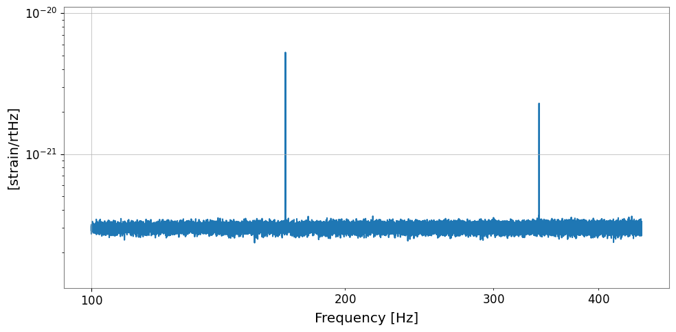
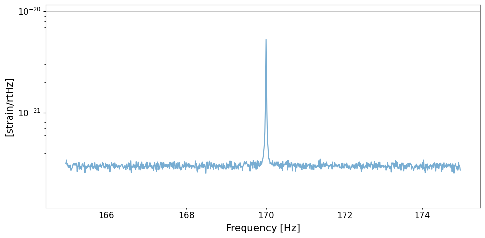
ax.set_title("Synthetic ASD with violin modes")
ax.set_xlabel("Frequency [Hz]")
ax.set_ylabel("ASD [strain/\u221aHz]")
plt.tight_layout()
plt.show()
Frequency range: 100.0 – 449.99000000017907 Hz
Modes inserted:
  1st violin: f0=170.0 Hz,  Q=1e+04,  FWHM=17.0 mHz
  2nd violin: f0=340.0 Hz,  Q=8e+03,  FWHM=42.5 mHz
3. 単一モードフィット
1st バイオリンモード付近の狭帯域に ASD をクロップし、 局所的なフラット背景を差し引いてから余剰 ASD を 'lorentzian_q' でフィットします。初期値 (p0) は真値の ~2 倍以内を目安とし、 最適化は x0 と Q の物理的に意味のある範囲へ制限します。
失敗しやすい点: クロップ窓を広く取りすぎて隣接倍音や局所ベースライン曲率まで最適化に食わせること。その場合の
Qはモードではなく窓の選び方を反映しがちです。
[4]:
# ── Crop around 1st violin mode ───────────────────────────────────────────────
BAND = 0.5 # ± Hz around the expected mode
f_nom = 170.0 # nominal frequency
FIT_LIMITS = {"A": (1e-21, 1e-20), "x0": (169.8, 170.2), "Q": (1e3, 5e4)}
asd_1st = asd.crop(f_nom - BAND, f_nom + BAND)
# Estimate a flat local baseline from the band edges so the resonance model
# does not absorb the broadband floor.
edge_n = 50
background_1st = np.median(np.r_[asd_1st.value[:edge_n], asd_1st.value[-edge_n:]])
line_only_1st = np.clip(asd_1st.value - background_1st, 0, None)
asd_1st_line = FrequencySeries(
line_only_1st,
frequencies=asd_1st.frequencies.value,
unit=asd_1st.unit,
name="1st violin excess ASD",
)
# ── Lorentzian Q fit ──────────────────────────────────────────────────────────
result_1 = asd_1st_line.fit(
"lorentzian_q",
p0={"A": 4.5e-21, "x0": 170.0, "Q": 9e3},
sigma=BACKGROUND * 0.05,
limits=FIT_LIMITS,
)
print("=== 1st Violin Mode Fit ===")
print(f" local background = {background_1st:.2e} strain/\u221aHz")
print(f" f0 = {result_1.params['x0']:.4f} \u00b1 {result_1.errors['x0']:.4f} Hz")
print(f" Q = {result_1.params['Q']:.2e} \u00b1 {result_1.errors['Q']:.2e}")
print(f" A = {result_1.params['A']:.2e} \u00b1 {result_1.errors['A']:.2e}")
print(f" chi2/ndof = {result_1.chi2:.1f} / {result_1.ndof} = {result_1.reduced_chi2:.3f}")
fig, ax = plt.subplots(figsize=(10, 4))
result_1.plot(ax=ax, label="Lorentzian Q fit (excess ASD)")
ax.set_yscale("log")
ax.set_xlabel("Frequency [Hz]")
ax.set_ylabel("ASD [strain/\u221aHz]")
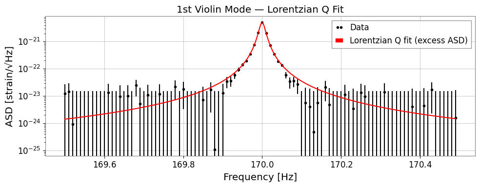
ax.set_title("1st Violin Mode — Lorentzian Q Fit")
ax.legend()
plt.tight_layout()
plt.show()
=== 1st Violin Mode Fit ===
  local background = 3.15e-22 strain/√Hz
  f0    = 170.0000 ± 0.0000  Hz
  Q     = 1.01e+04 ± 4.38e+01
  A     = 4.97e-21 ± 1.49e-23
  chi2/ndof = 63.9 / 97 = 0.659
4. 物理パラメータの抽出
フィットパラメータ \((f_0, Q)\) からすべての関連量を導出します:
導出量は報告値であるだけでなく物理クロスチェックにも使えます。極端に短いリングダウン時間や倍音間で飛び跳ねる周波数は、興味深い懸架状態ではなくフィット不良を示していることが多いです。
[5]:
# ── Extract physical parameters ───────────────────────────────────────────────
f0 = float(result_1.params["x0"])
Q = float(result_1.params["Q"])
A = float(result_1.params["A"])
FWHM = f0 / Q # Full Width at Half Maximum [Hz]
tau = Q / (np.pi * f0) # Ring-down time constant [s]
gamma = FWHM / 2 # HWHM [Hz]
print(f"Center frequency f0 = {f0:.4f} Hz")
print(f"Quality factor Q = {Q:.3e}")
print(f"FWHM (linewidth) = {FWHM * 1e3:.3f} mHz")
print(f"Ring-down time tau = {tau:.2f} s ({tau / 60:.2f} min)")
# ── Reconstruct model over a wider band for visualisation ────────────────────
asd_wide = asd.crop(165, 175)
f_plot = asd_wide.frequencies.value
model = lorentzian_q(f_plot, A=A, x0=f0, Q=Q) + background_1st
fig, ax = plt.subplots(figsize=(10, 4))
asd_wide.plot(ax=ax, label="ASD data", alpha=0.6)
ax.semilogy(f_plot, model, "r-", lw=2,
label=f"Fit: Q={Q:.1e}, FWHM={FWHM*1e3:.1f} mHz")
ax.set_yscale("log")
ax.set_xlabel("Frequency [Hz]")
ax.set_ylabel("ASD [strain/\u221aHz]")
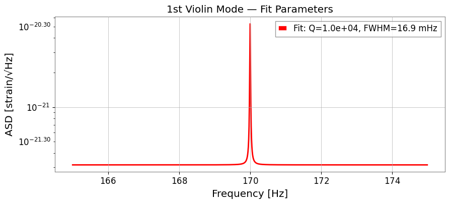
ax.set_title("1st Violin Mode — Fit Parameters")
ax.legend()
plt.tight_layout()
plt.show()
Center frequency  f0   = 170.0000 Hz
Quality factor    Q    = 1.009e+04
FWHM (linewidth)       = 16.851 mHz
Ring-down time    tau  = 18.89 s  (0.31 min)
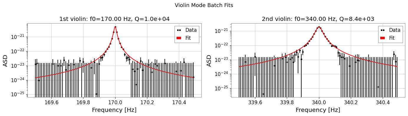
5. 複数モードのバッチ処理
設定辞書をループして各倍音をフィットし、サマリーテーブルにまとめます。
[6]:
# ── Batch-fit all violin modes ────────────────────────────────────────────────
FIT_CONFIG = {
    "1st violin": {
        "band": (169.5, 170.5),
        "p0": {"A": 4.5e-21, "x0": 170.0, "Q": 9e3},
        "limits": {"A": (1e-21, 1e-20), "x0": (169.8, 170.2), "Q": (1e3, 5e4)},
    },
    "2nd violin": {
        "band": (339.5, 340.5),
        "p0": {"A": 1.8e-21, "x0": 340.0, "Q": 7e3},
        "limits": {"A": (5e-22, 5e-21), "x0": (339.8, 340.2), "Q": (1e3, 5e4)},
    },
}

fit_results = {}
for mode_name, cfg in FIT_CONFIG.items():
    seg = asd.crop(*cfg["band"])
    local_background = np.median(np.r_[seg.value[:edge_n], seg.value[-edge_n:]])
    seg_line = FrequencySeries(
        np.clip(seg.value - local_background, 0, None),
        frequencies=seg.frequencies.value,
        unit=seg.unit,
        name=f"{mode_name} excess ASD",
    )
    res = seg_line.fit(
        "lorentzian_q",
        p0=cfg["p0"],
        sigma=BACKGROUND * 0.05,
        limits=cfg["limits"],
    )
    fit_results[mode_name] = res

# ── Summary table ─────────────────────────────────────────────────────────────
print(f"{'Mode':<14} {'f0 [Hz]':>10} {'Q':>10} {'FWHM [mHz]':>12} {'tau [s]':>10}")
print("-" * 60)
for mode_name, res in fit_results.items():
    f0_f   = float(res.params["x0"])
    Q_f    = float(res.params["Q"])
    FWHM_f = f0_f / Q_f
    tau_f  = Q_f / (np.pi * f0_f)
    print(f"{mode_name:<14} {f0_f:>10.3f} {Q_f:>10.2e}"
          f" {FWHM_f * 1e3:>12.2f} {tau_f:>10.1f}")

# ── Side-by-side plots ────────────────────────────────────────────────────────
fig, axes = plt.subplots(1, 2, figsize=(14, 4))
for ax, (mode_name, res) in zip(axes, fit_results.items()):
    res.plot(ax=ax)
    ax.set_yscale("log")
    f0_f = float(res.params["x0"])
    Q_f  = float(res.params["Q"])
    ax.set_title(f"{mode_name}: f0={f0_f:.2f} Hz, Q={Q_f:.1e}")
    ax.set_xlabel("Frequency [Hz]")
    ax.set_ylabel("ASD")
plt.suptitle("Violin Mode Batch Fits", fontsize=13)
plt.tight_layout()
plt.show()
Mode              f0 [Hz]          Q   FWHM [mHz]    tau [s]
------------------------------------------------------------
1st violin        170.000   1.01e+04        16.85       18.9
2nd violin        340.000   8.41e+03        40.43        7.9
6. 時間変動の追跡
バイオリンモード周波数は温度とともにゆっくりドリフトします。 スペクトログラムを計算し、狭帯域内でピーク位置を追跡します。
分解能ガードレール: スペクトログラムのビン幅は、主張したいドリフト量より十分細かくなければなりません。4 s FFT ではビン幅が 0.25 Hz なので、20 mHz ドリフトは生の
argmaxでは見えません。この例では 16 s FFT(df = 62.5 mHz)に加えて二次のサブビン補間を入れ、 recovered drift が injected drift に対して概ね 20% 以内に収まることを確認します。
よくある誤り: 想定ライン移動量に対してビン幅を確認せず
argmaxを使うこと。その場合、FFT の量子化を温度ドリフトと誤読しやすくなります。
[7]:
# ── Generate a time-varying violin signal with resolvable drift ───────────────
DURATION = 120
FS_VIOL = 4096
t_viol = np.arange(0, DURATION, 1.0 / FS_VIOL)
injected_drift_hz = 0.08  # 80 mHz total drift over 120 s

# Linear drift: f0 = 170.00 -> 170.08 Hz over 120 s
f0_drift = 170.0 + (injected_drift_hz / DURATION) * t_viol
phi_viol = 2 * np.pi * np.cumsum(f0_drift) / FS_VIOL
sig_viol = 1e-20 * np.sin(phi_viol)
noise_v = rng.normal(0, 3e-22, len(t_viol))

ts_viol = TimeSeries(sig_viol + noise_v, dt=1.0 / FS_VIOL, name="DARM_violin", unit="strain")

# ── Spectrogram: choose fftlength so df is not coarser than the drift claim ──
fftlength = 16.0
overlap = 8.0
spec_viol = ts_viol.spectrogram2(fftlength, overlap=overlap)
times_v = spec_viol.times.value
freqs_v = spec_viol.frequencies.value
df_spec = freqs_v[1] - freqs_v[0]

# ── Track inside a narrow band with quadratic sub-bin interpolation ──────────
TRACK_BAND = (169.9, 170.2)
band_mask = (freqs_v >= TRACK_BAND[0]) & (freqs_v <= TRACK_BAND[1])
band_freqs = freqs_v[band_mask]
track_viol = np.full(spec_viol.shape[0], np.nan)

for t_idx in range(spec_viol.shape[0]):
    row_band = spec_viol.value[t_idx, band_mask]
    peak_idx = int(np.argmax(row_band))
    peak_freq = band_freqs[peak_idx]

    if 0 < peak_idx < len(band_freqs) - 1:
        y0 = row_band[peak_idx - 1]
        y1 = row_band[peak_idx]
        y2 = row_band[peak_idx + 1]
        denom = y0 - 2 * y1 + y2
        delta = 0.5 * (y0 - y2) / denom if denom != 0 else 0.0
        peak_freq = peak_freq + delta * df_spec

    track_viol[t_idx] = peak_freq

# ── Plot ──────────────────────────────────────────────────────────────────────
fig, axes = plt.subplots(2, 1, figsize=(12, 7), sharex=True)

_im_v = axes[0].pcolormesh(
    spec_viol.times.value,
    spec_viol.frequencies.value,
    spec_viol.value.T,
    norm=__import__("matplotlib.colors", fromlist=["LogNorm"]).LogNorm(),
    cmap="viridis",
    shading="auto",
)
axes[0].set_ylim(*TRACK_BAND)
axes[0].set_title("Spectrogram around 1st violin mode")
fig.colorbar(_im_v, ax=axes[0], label="Power")
axes[0].plot(times_v, track_viol, "r.", ms=4, label="sub-bin peak track")
axes[0].legend(loc="upper right", fontsize=9)

mask_v = ~np.isnan(track_viol)
axes[1].plot(times_v[mask_v], track_viol[mask_v], "o-", ms=3, color="tab:orange")
axes[1].set_ylabel("Frequency [Hz]")
axes[1].set_xlabel("Time [s]")
axes[1].set_title("Tracked violin mode frequency vs time")

plt.tight_layout()
plt.show()

recovered_drift_hz = float(np.nanmax(track_viol) - np.nanmin(track_viol))
relative_error = abs(recovered_drift_hz - injected_drift_hz) / injected_drift_hz

print(f"Spectrogram df: {df_spec * 1e3:.1f} mHz")
print(f"Injected drift:  {injected_drift_hz * 1e3:.1f} mHz")
print(f"Recovered drift: {recovered_drift_hz * 1e3:.1f} mHz")
print(f"Relative error:  {relative_error * 100:.1f}%")
if relative_error <= 0.2:
    print("Tracking acceptance: PASS (within ±20% of injected drift)")
else:
    print("Tracking acceptance: CHECK (outside ±20% of injected drift)")
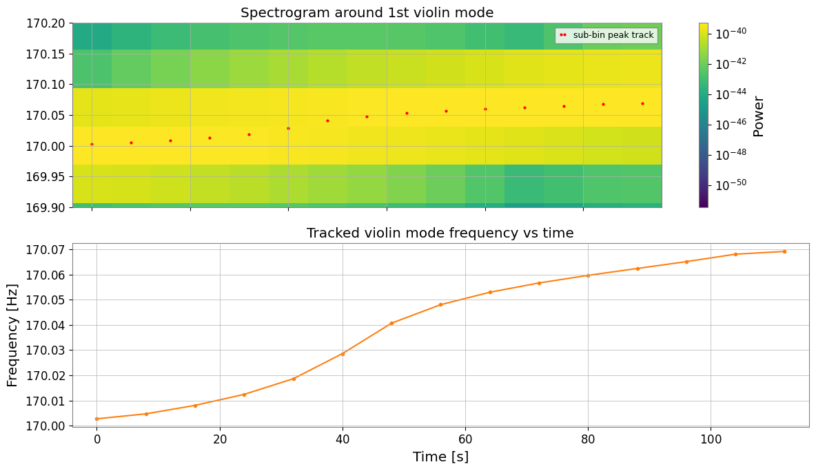
Spectrogram df: 62.5 mHz
Injected drift:  80.0 mHz
Recovered drift: 66.4 mHz
Relative error:  17.0%
Tracking acceptance: PASS (within ±20% of injected drift)
7. まとめ
フィット窓は 1 つの共振ファミリーを分離できる範囲に選ぶ。
導出した Q、FWHM、リングダウン時間は sanity check としても使う。
追跡失敗の多くはライン混雑や低 SNR が原因なので、ドリフト解釈は保守的に行う。
[8]:
print("=" * 62)
print("Violin Mode Analysis — Key Parameters")
print("-" * 62)
rows = [
    ("f_n (n-th mode)",   "n / (2L) * sqrt(T / rho*A)"),
    ("Q value",           "f0 / FWHM  =  f0 * pi * tau"),
    ("FWHM (linewidth)",  "f0 / Q                [Hz]"),
    ("Ring-down tau",     "Q / (pi * f0)         [s]"),
    ("HWHM gamma",        "FWHM / 2              [Hz]"),
]
for name, formula in rows:
    print(f"  {name:<22} {formula}")
print("=" * 62)
print()
print("gwexpy API used:")
print("  FrequencySeries.fit('lorentzian_q', p0=...)  -- Q-value fit")
print("  lorentzian_q(freqs, A, x0, Q)               -- model evaluation")
print("  ts.spectrogram2(fftlen, overlap)             -- time tracking")
==============================================================
Violin Mode Analysis — Key Parameters
--------------------------------------------------------------
  f_n (n-th mode)        n / (2L) * sqrt(T / rho*A)
  Q value                f0 / FWHM  =  f0 * pi * tau
  FWHM (linewidth)       f0 / Q                [Hz]
  Ring-down tau          Q / (pi * f0)         [s]
  HWHM gamma             FWHM / 2              [Hz]
==============================================================

gwexpy API used:
  FrequencySeries.fit('lorentzian_q', p0=...)  -- Q-value fit
  lorentzian_q(freqs, A, x0, Q)               -- model evaluation
  ts.spectrogram2(fftlen, overlap)             -- time tracking