Case navigation:
Back to the canonical gallery: Case Studies
Related reference surfaces: Reference Index, API: Matrix Containers, API: Frequency Series
Neighboring featured workflows: Noise Budgeting, Transfer Function Measurement
Active Damping for 6-DOF Active Vibration Isolation System (Non-Collocated Configuration)#
This tutorial demonstrates an end-to-end workflow combining gwexpy and python-control to perform simulation, system identification, and control design for a multi-degree-of-freedom (MIMO) system.
Scenario: We consider an equilateral triangular vibration isolation platform supported by three legs (6-DOF rigid body). In this case, we deal with a non-collocated configuration where actuators and sensors are located at different positions.
Actuators: Located at the three leg positions (support points) at \(0^\circ, 120^\circ, 240^\circ\)
Sensors: Located at mid-points between the legs at \(60^\circ, 180^\circ, 300^\circ\)
When the input/output positions are misaligned like this, simple independent control for each axis does not work well. Therefore, we perform controller design in Modal Space.
Steps:
Physical Model Construction: Create a state-space model considering sensor and actuator placement.
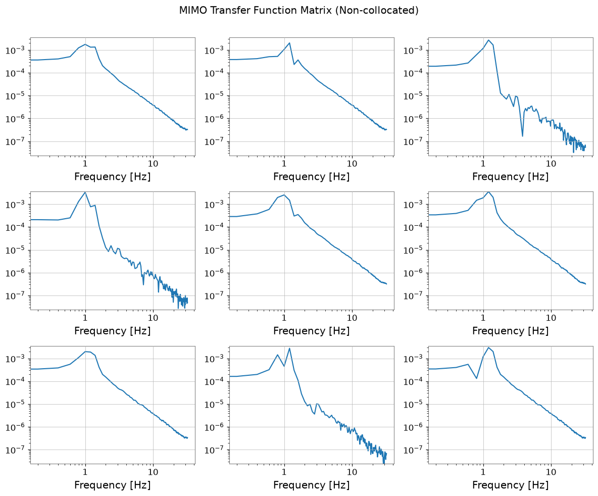
MIMO Transfer Function Measurement: Visualize the transfer function matrix including off-diagonal components using
FrequencySeriesMatrix.System Identification: Define a control model from physical parameters and geometric configuration.
Damping Controller Design: Design “modal control” that converts sensor signals to modal coordinates and applies damping to each mode.
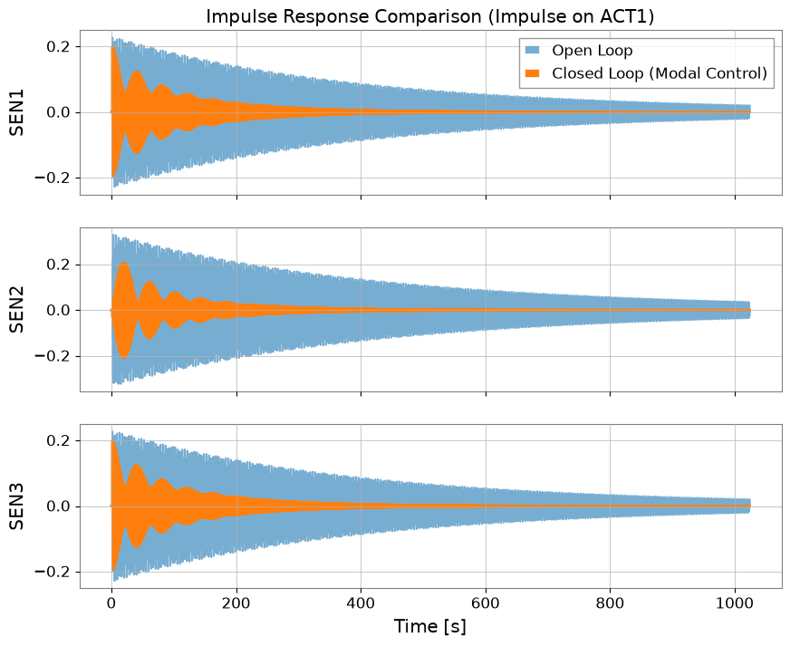
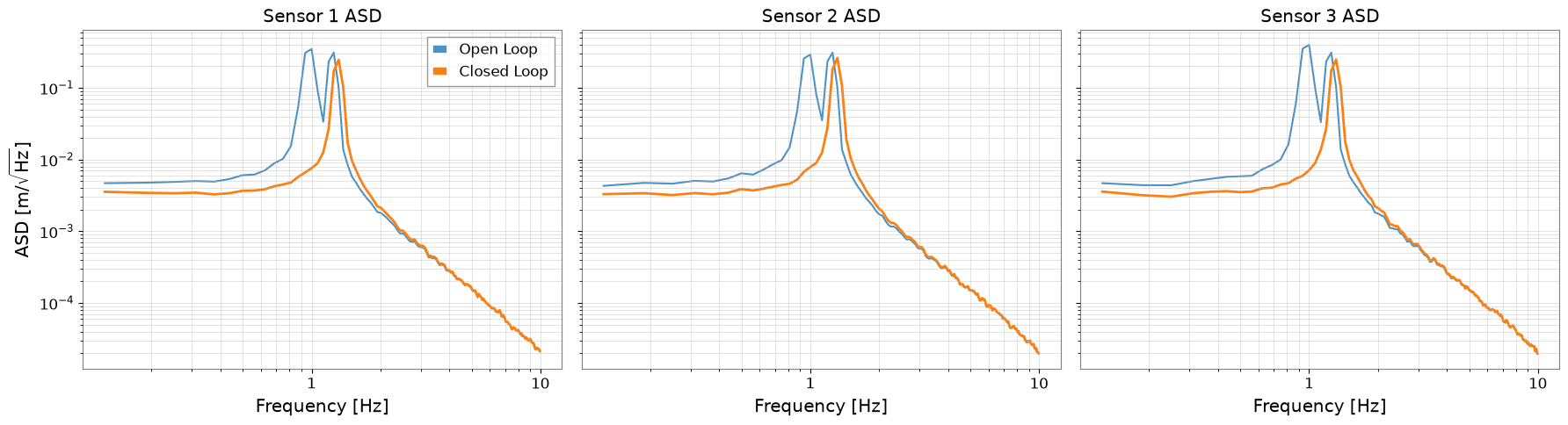
Closed-Loop Verification: Confirm vibration suppression performance through impulse response and ASD comparison.
import warnings


import control
import matplotlib.pyplot as plt
import numpy as np
from scipy import signal

from gwexpy import TimeSeries, TimeSeriesDict
from gwexpy.frequencyseries import FrequencySeriesMatrix
1. Simulation of 6-DOF Active Vibration Isolation System (Plant Model)#
We define the rigid body equation of motion \(M \ddot{q} + C \dot{q} + K q = F\). Here we focus on the three vertical degrees of freedom (\(z, \theta_x, \theta_y\)).
Coordinate Transformation: For modal coordinates \(q = [z, \theta_x, \theta_y]^T\),
Actuator physical coordinates \(p_{act}\): \(0^\circ, 120^\circ, 240^\circ\)
Sensor physical coordinates \(p_{sen}\): \(60^\circ, 180^\circ, 300^\circ\)
We define the transformation matrices \(T_{act}, T_{sen}\) for each and incorporate them into the state-space model.
# Physical parameters for the rigid-body modes we want to damp: one vertical translation and two tilts.
m = 100.0  # mass [kg]
I_x = 20.0  # moment of inertia [kg m^2]
I_y = 20.0

# Springs and dampers act at the leg locations, so their stiffness and loss enter through actuator-space geometry.
k_leg = 2000.0  # spring constant [N/m]
c_leg = 0.20  # damping coefficient [N s/m]

# Geometry sets how vertical motion mixes into pitch/roll; that lever arm is what creates modal cross-coupling.
R = 0.5  # [m]

# Define actuator and sensor placement separately so we can study the non-collocated case.
deg2rad = np.pi / 180.0
# Actuators push at the support legs.
angles_act = np.array([0, 120, 240]) * deg2rad
# Sensors are intentionally offset from the actuators, which is why a naive diagonal controller would mix modes.
angles_sen = np.array([60, 180, 300]) * deg2rad


# Build the geometry matrix that maps rigid-body modal coordinates into physical sensor/actuator displacements.
# Each row says how one leg/sensor displacement is produced by vertical motion plus pitch/roll about the platform center.
def make_transform_matrix(angles, radius):
    T = np.zeros((3, 3))
    for i, ang in enumerate(angles):
        T[i, 0] = 1.0
        T[i, 1] = radius * np.sin(ang)
        T[i, 2] = -radius * np.cos(ang)
    return T


T_act = make_transform_matrix(angles_act, R)
T_sen = make_transform_matrix(angles_sen, R)

print("Actuator Transform Matrix T_act:")
print(np.round(T_act, 2))
print("Sensor Transform Matrix T_sen:")
print(np.round(T_sen, 2))

# Mass/inertia stay diagonal in modal coordinates, which makes the physical rigid-body modes easy to interpret.
M_modal = np.diag([m, I_x, I_y])

# Stiffness and damping start in leg space because that is where the hardware is attached.
K_phys = np.diag([k_leg, k_leg, k_leg])
C_phys = np.diag([c_leg, c_leg, c_leg])

# Project stiffness/damping into modal space so translation and rotations can be controlled as separate physical modes.
# Use the actuator geometry here because the restoring forces are applied at the legs, not at the sensor locations.
K_modal = T_act.T @ K_phys @ T_act
C_modal = T_act.T @ C_phys @ T_act

# Build the plant in state space so open-loop and closed-loop motion can be compared with the same model.
# x = [q, q_dot]^T
A_sys = np.block(
    [
        [np.zeros((3, 3)), np.eye(3)],
        [-np.linalg.inv(M_modal) @ K_modal, -np.linalg.inv(M_modal) @ C_modal],
    ]
)
B_sys_modal = np.block([[np.zeros((3, 3))], [np.linalg.inv(M_modal)]])
C_sys_modal = np.block([np.eye(3), np.zeros((3, 3))])
D_sys = np.zeros((3, 3))

# Convert between modal and physical coordinates because hardware talks in leg forces and sensor displacements, not pure modes.
# Input: Actuator forces u at leg locations -> generalized modal force Q = T_act.T * u
# Output: Sensor displacements y at sensor locations -> y = T_sen * q
B_sys = B_sys_modal @ T_act.T
C_sys = T_sen @ C_sys_modal

sys = control.StateSpace(
    A_sys,
    B_sys,
    C_sys,
    D_sys,
    inputs=["ACT1", "ACT2", "ACT3"],
    outputs=["SEN1", "SEN2", "SEN3"],
)
print(sys)
Actuator Transform Matrix T_act:
[[ 1.    0.   -0.5 ]
 [ 1.    0.43  0.25]
 [ 1.   -0.43  0.25]]
Sensor Transform Matrix T_sen:
[[ 1.    0.43 -0.25]
 [ 1.    0.    0.5 ]
 [ 1.   -0.43 -0.25]]
<StateSpace>: sys[0]
Inputs (3): ['ACT1', 'ACT2', 'ACT3']
Outputs (3): ['SEN1', 'SEN2', 'SEN3']
States (6): ['x[0]', 'x[1]', 'x[2]', 'x[3]', 'x[4]', 'x[5]']

A = [[ 0.00000000e+00  0.00000000e+00  0.00000000e+00
       1.00000000e+00  0.00000000e+00  0.00000000e+00]
     [ 0.00000000e+00  0.00000000e+00  0.00000000e+00
       0.00000000e+00  1.00000000e+00  0.00000000e+00]
     [ 0.00000000e+00  0.00000000e+00  0.00000000e+00
       0.00000000e+00  0.00000000e+00  1.00000000e+00]
     [-6.00000000e+01 -3.33955086e-15 -2.16715534e-15
      -6.00000000e-03 -3.68259567e-19 -2.35922393e-19]
     [-1.70530257e-14 -3.75000000e+01  9.61481343e-15
      -2.08166817e-18 -3.75000000e-03  9.61481343e-19]
     [-1.13686838e-14  9.93438680e-15 -3.75000000e+01
      -1.04083409e-18  9.61481343e-19 -3.75000000e-03]]

B = [[ 0.          0.          0.        ]
     [ 0.          0.          0.        ]
     [ 0.          0.          0.        ]
     [ 0.01        0.01        0.01      ]
     [ 0.          0.02165064 -0.02165064]
     [-0.025       0.0125      0.0125    ]]

C = [[ 1.00000000e+00  4.33012702e-01 -2.50000000e-01
       0.00000000e+00  0.00000000e+00  0.00000000e+00]
     [ 1.00000000e+00  6.12323400e-17  5.00000000e-01
       0.00000000e+00  0.00000000e+00  0.00000000e+00]
     [ 1.00000000e+00 -4.33012702e-01 -2.50000000e-01
       0.00000000e+00  0.00000000e+00  0.00000000e+00]]

D = [[0. 0. 0.]
     [0. 0. 0.]
     [0. 0. 0.]]
2. MIMO Transfer Function Measurement#
Since the sensor and actuator positions differ, strong responses should appear not only in the diagonal components (ACT1->SEN1) but also in the off-diagonal components.
fs = 64
duration = 1024.0
t = np.arange(0, duration, 1 / fs)
n_samples = len(t)

# Drive all three actuators with broadband excitation so every mode is visible in the measured MIMO transfer matrix.
np.random.seed(0)
u_data = np.random.normal(0, 1.0, (3, n_samples))

# Simulate the plant response to that broadband drive, mimicking a system-identification experiment.
time_response = control.forced_response(sys, T=t, U=u_data)

# Wrap channels as TimeSeriesDict so transfer estimation uses the same workflow as measured detector data.
tsd_input = TimeSeriesDict(
    {
        f"ACT{i + 1}": TimeSeries(
            u_data[i], t0=0, sample_rate=fs, name=f"Actuator {i + 1}", unit="N"
        )
        for i in range(3)
    }
)

tsd_output = TimeSeriesDict.from_control(time_response, unit="m")
for i in range(3):
    tsd_output[f"SEN{i + 1}"].name = f"Sensor {i + 1}"

# Estimate the full 3x3 transfer matrix to reveal how each actuator leaks into every sensor in the non-collocated layout.
tfs = [
    [
        tsd_input[f"ACT{j + 1}"].transfer_function(
            tsd_output[f"SEN{i + 1}"], fftlength=5
        )
        for j in range(3)
    ]
    for i in range(3)
        ]

tf_matrix = FrequencySeriesMatrix(
    [[tf.value for tf in row] for row in tfs], frequencies=tfs[0][0].frequencies
)

tf_data = tf_matrix.value
freqs = tf_matrix.frequencies

# Plot the matrix magnitude to see both the dominant resonant paths and the off-diagonal cross-couplings that modal control must suppress.
tf_matrix.abs().plot(figsize=(12, 10), xscale="log", yscale="log").suptitle(
    "MIMO Transfer Function Matrix (Non-collocated)\n"
)
plt.tight_layout()
plt.show()
3 & 4. Modal Control Design#
Since the actuator and sensor positions do not coincide, simple decentralized control (\(F_i \propto \dot{y}_i\)) may become unstable. Therefore, we adopt a method that estimates modal displacement from sensor signals using transformation matrices, applies damping in modal space, and then distributes the result to actuator forces.
Control Flow:
Sensing: Estimate modal displacement \(q\) from sensor output \(y\) $\( q_{est} = T_{sen}^{-1} y \)$
Modal Damping: Apply pseudo-derivative filter \(K(s)\) to each mode to calculate modal force \(F_{modal}\) $\( F_{modal} = -K_{modal}(s) q_{est} \)$
Actuation: Distribute modal force \(F_{modal}\) to actuator forces \(u\) $\( u = (T_{act}^T)^{-1} F_{modal} \)$
Overall, the MIMO controller \(K_{MIMO}\) becomes: $\( K_{MIMO}(s) = (T_{act}^T)^{-1} \cdot \mathrm{diag}(K_{z}(s), K_{\theta x}(s), K_{\theta y}(s)) \cdot T_{sen}^{-1} \)$
# --- 1. Prepare sensing/actuation transforms so the controller works in modal coordinates instead of raw sensor space. ---
# In practice these come from an identified plant; here we use the true geometry to isolate the control concept.
# Sensor signals are mixed estimates of the rigid-body modes, so invert that geometry first.
S_sensing = np.linalg.inv(T_sen)

# Modal forces must be mapped back to physical actuator commands before the hardware can realize them.
# F_modal = T_act.T * u  =>  u = inv(T_act.T) * F_modal
D_actuation = np.linalg.inv(T_act.T)

print("Sensing Matrix (Sensor -> Mode):")
print(np.round(S_sensing, 2))
print("Actuation Matrix (Mode Force -> Actuator):")
print(np.round(D_actuation, 2))

# --- 2. Design a modal damping filter that targets resonance energy instead of raw sensor motion. ---
# Gains are chosen in modal coordinates so each rigid-body resonance can be damped without feeding back the wrong combination of sensors.
# Translation and tilt could need different gains because their masses/inertias differ,
# but this example keeps them equal to highlight the geometry rather than controller tuning.
gain = 1000.0  # Modal damping gain
fc_l = 0.1
fc_h = 20.0
w_l = 2 * np.pi * fc_l
w_h = 2 * np.pi * fc_h

s = control.tf("s")
K_filter = gain * s / ((1 + s / w_l) * (1 + s / w_h))

# A diagonal modal controller means each mode is damped independently once the geometry has been unmixed.
K_modal_diag = []
for _ in range(3):
    K_modal_diag.append(control.ss(K_filter))

# control.append builds the three independent modal filters into one block-diagonal system.
# Keeping the blocks separate avoids accidentally re-introducing artificial cross-coupling in the controller model.
# python-control then handles the series products needed to move back into actuator space.
K_modal_block = control.append(K_modal_diag[0], K_modal_diag[1], K_modal_diag[2])


# --- 3. Reassemble the controller in physical coordinates so the hardware sees actuator commands but the feedback law still damps modal motion. ---
# Multiplication order matters because a mistaken order would mix sensors and actuators incorrectly, creating non-physical feedback paths.
# The intended flow is measured sensor motion -> modal coordinates -> modal damping law -> actuator commands.
K_mimo = D_actuation * K_modal_block * S_sensing

print("MIMO Controller States:", K_mimo.nstates)
Sensing Matrix (Sensor -> Mode):
[[ 0.33  0.33  0.33]
 [ 1.15 -0.   -1.15]
 [-0.67  1.33 -0.67]]
Actuation Matrix (Mode Force -> Actuator):
[[ 0.33 -0.   -1.33]
 [ 0.33  1.15  0.67]
 [ 0.33 -1.15  0.67]]
MIMO Controller States: 6
5 & 6. Closed-Loop Verification (Impulse Response & ASD)#
Using the constructed modal control system, we perform closed-loop simulation. We verify the response to an impulse disturbance on actuator 1 and to steady-state ground vibration on all axes.
# Close the loop and compare it with open loop to see whether modal damping reduces the resonant motion.
sys_cl = control.feedback(sys, K_mimo, sign=-1)

# --- Impulse response shows how quickly a localized actuator kick rings down with and without modal damping. ---
u_impulse = np.zeros((3, n_samples))
u_impulse[0, 100] = 100.0 * fs  # Impulse on actuator 1

resp_ol = control.forced_response(sys, T=t, U=u_impulse)
resp_cl = control.forced_response(sys_cl, T=t, U=u_impulse)

fig, axes = plt.subplots(3, 1, figsize=(10, 8), sharex=True)
for i in range(3):
    ax = axes[i]
    ax.plot(t, resp_ol.outputs[i], label="Open Loop", alpha=0.6)
    ax.plot(t, resp_cl.outputs[i], label="Closed Loop (Modal Control)", linewidth=2)
    ax.set_ylabel(f"SEN{i + 1}")
    ax.grid(True)
    if i == 0:
        ax.legend(loc="upper right")
axes[2].set_xlabel("Time [s]")
axes[0].set_title("Impulse Response Comparison (Impulse on ACT1)")
plt.show()

# --- ASD comparison asks whether the controller lowers the disturbance-driven motion across the resonance band. ---
# Use low-frequency ground-like disturbance so the rigid-body resonance is excited in the same band the controller is meant to suppress.
np.random.seed(42)
wn = np.random.normal(0, 1.0, (3, n_samples))
b, a = signal.butter(1, 5.0, fs=fs, btype="low")
dist = signal.lfilter(b, a, wn) * 50.0

resp_ol_noise = control.forced_response(sys, T=t, U=dist)
resp_cl_noise = control.forced_response(sys_cl, T=t, U=dist)

tsd_ol = TimeSeriesDict.from_control(resp_ol_noise)
for i in range(3):
    tsd_ol[list(tsd_ol.keys())[i]].name = f"SEN{i + 1}"
tsd_ol = TimeSeriesDict({ts.name: ts for ts in tsd_ol.values()})
tsd_cl = TimeSeriesDict.from_control(resp_cl_noise)
for i in range(3):
    tsd_cl[list(tsd_cl.keys())[i]].name = f"SEN{i + 1}"
tsd_cl = TimeSeriesDict({ts.name: ts for ts in tsd_cl.values()})

fig, axes = plt.subplots(1, 3, figsize=(18, 5), sharey=True)
for i in range(3):
    ax = axes[i]
    asd_ol = (
        tsd_ol[f"SEN{i + 1}"].asd(fftlength=16, overlap=8, method="welch").crop(0.1, 10)
    )
    asd_cl = (
        tsd_cl[f"SEN{i + 1}"].asd(fftlength=16, overlap=8, method="welch").crop(0.1, 10)
    )

    ax.loglog(asd_ol, label="Open Loop", alpha=0.8)
    ax.loglog(asd_cl, label="Closed Loop", linewidth=2)
    ax.set_title(f"Sensor {i + 1} ASD")
    ax.set_xlabel("Frequency [Hz]")
    ax.grid(True, which="both", alpha=0.5)
    if i == 0:
        ax.set_ylabel(r"ASD [$\mathrm{m}/\sqrt{\mathrm{Hz}}$]")
        ax.legend()
plt.tight_layout()
plt.show()

# Even with non-collocated sensors and actuators, the modal transforms let us damp the physical rigid-body modes instead of fighting geometry-induced cross-coupling directly in sensor space.