Development documentation · 0.2.3 30c2f8ba · Intro examples tested with 0.2.3 · Version details · Known limitations

Peak Tracking: Time Evolution

This tutorial extends advanced_peak_detection.ipynb by showing how to track spectral lines through time using a spectrogram.

Real-world examples:

• Power-line harmonics drifting with mains frequency

• Violin-mode resonances shifting with temperature

• Calibration lines with intentional frequency modulation

Strategy: compute a spectrogram → detect peaks per frame → connect with nearest-neighbour algorithm.

import warnings


import matplotlib.pyplot as plt
import numpy as np
from scipy.signal import find_peaks as sp_find_peaks

from gwexpy.timeseries import TimeSeries

plt.rcParams["figure.figsize"] = (12, 4)

1. Synthetic Data

Two spectral lines embedded in white Gaussian noise:

Line	Behaviour	Amplitude
1	58 → 62 Hz linear drift	0.5
2	120 Hz ± 0.5 Hz sinusoidal wobble	0.3

rng = np.random.default_rng(0)

DURATION = 120   # s
FS       = 512   # Hz
t = np.arange(0, DURATION, 1 / FS)

# ── Line 1: linear drift 58 → 62 Hz ──────────────────────────────────────────
f1_t   = 58.0 + (4.0 / DURATION) * t          # frequency as a function of t
phi1   = 2 * np.pi * np.cumsum(f1_t) / FS      # instantaneous phase
s1     = 0.5 * np.sin(phi1)

# ── Line 2: 120 Hz with slow sinusoidal wobble ±0.5 Hz ───────────────────────
f2_t   = 120.0 + 0.5 * np.sin(2 * np.pi * 0.03 * t)
phi2   = 2 * np.pi * np.cumsum(f2_t) / FS
s2     = 0.3 * np.sin(phi2)

# ── Background Gaussian noise ────────────────────────────────────────────────
noise = rng.normal(0, 0.05, len(t))

strain = s1 + s2 + noise
ts = TimeSeries(strain, dt=1.0 / FS, name="STRAIN", unit="strain")

print(f"Duration : {DURATION} s   |  Sample rate: {FS} Hz")
print("Line 1   : 58 → 62 Hz (linear drift)")
print("Line 2   : 120 Hz ± 0.5 Hz (slow wobble)")

Duration : 120 s   |  Sample rate: 512 Hz
Line 1   : 58 → 62 Hz (linear drift)
Line 2   : 120 Hz ± 0.5 Hz (slow wobble)

2. Spectrogram Overview

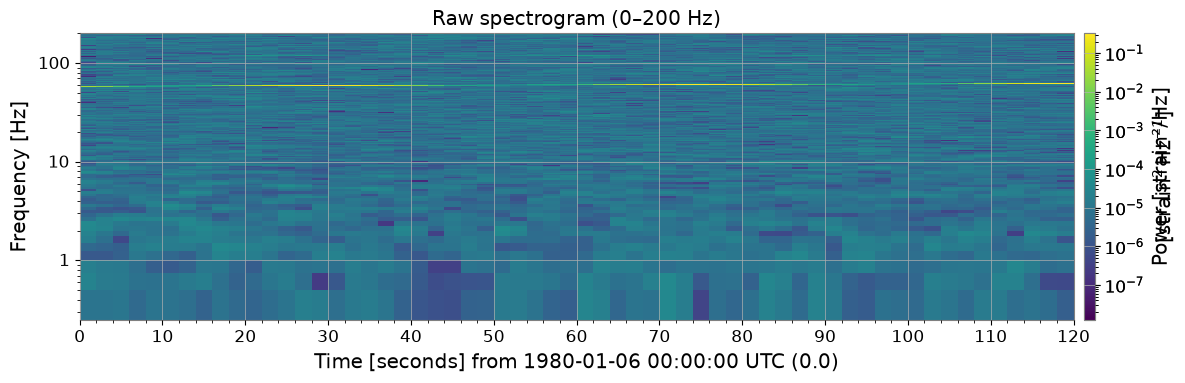
ts.spectrogram2(fftlength, overlap) returns a time–frequency power map. The diagonal streak (Line 1 drift) and slightly wavy horizontal stripe (Line 2 wobble) are already visible.

import warnings

with warnings.catch_warnings():

    FFTLEN  = 4.0   # FFT length [s]
    OVERLAP = 2.0   # overlap [s]

    spec = ts.spectrogram2(FFTLEN, overlap=OVERLAP)
    print("Spectrogram shape (time × freq):", spec.shape)
    print(f"Time bins : {spec.shape[0]}  |  Freq bins: {spec.shape[1]}")
    print(f"Freq resolution: {spec.df.value:.4f} Hz")

    _plt_sp = spec.plot(norm="log", figsize=(12, 4))
    ax = _plt_sp.gca()
    fig = _plt_sp.figure
    ax.set_ylim(0, 200)
    ax.set_title("Raw spectrogram (0–200 Hz)")
    _plt_sp.colorbar(label="Power [strain²/Hz]")
    with warnings.catch_warnings():
        warnings.filterwarnings("ignore", message="This figure includes Axes that are not compatible with tight_layout")
    plt.tight_layout()
    plt.show()

Spectrogram shape (time × freq): (60, 1025)
Time bins : 60  |  Freq bins: 1025
Freq resolution: 0.2500 Hz

3. Frame-by-Frame Peak Detection

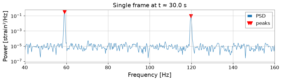
spec.value[t, :] is the 1-D PSD array at time index t. Pass it to scipy.signal.find_peaks with a height threshold and a minimum-distance constraint (in frequency bins).

import warnings

with warnings.catch_warnings():

    # ── Inspect one time frame ────────────────────────────────────────────────────
    T_IDX = spec.shape[0] // 4          # pick a time index near the 30-s mark
    row   = spec.value[T_IDX, :]        # PSD at this time
    freqs = spec.frequencies.value      # frequency axis [Hz]

    peaks_idx, props = sp_find_peaks(
    row,
    height=row.max() * 0.02,        # at least 2 % of frame maximum
    distance=int(5 / spec.df.value),# minimum 5 Hz separation
    )

    print(f"Time index {T_IDX}  (t ≈ {spec.times.value[T_IDX]:.1f} s)")
    print(f"Detected peaks at: {freqs[peaks_idx].round(2)} Hz")

    fig, ax = plt.subplots(figsize=(10, 3))
    ax.semilogy(freqs, row, lw=0.8, label="PSD")
    ax.semilogy(freqs[peaks_idx], row[peaks_idx], "rv", ms=8, label="peaks")
    ax.set_xlim(40, 160)
    ax.set_xlabel("Frequency [Hz]")
    ax.set_ylabel("Power [strain²/Hz]")
    ax.set_title(f"Single frame at t ≈ {spec.times.value[T_IDX]:.1f} s")
    ax.legend()
    with warnings.catch_warnings():
        warnings.filterwarnings("ignore", message="This figure includes Axes that are not compatible with tight_layout")
    plt.tight_layout()
    plt.show()

Time index 15  (t ≈ 30.0 s)
Detected peaks at: [ 59.   119.75] Hz

4. Single-Line Tracking (nearest-neighbour)

Algorithm

seed = initial frequency estimate
for each time frame t:
    detect all peaks in PSD(t)
    find the peak nearest to current seed
    if distance < max_jump:
        record that frequency
        update seed ← new frequency   # propagate
    else:
        record NaN                     # no detection

Updating the seed at each step lets the tracker follow a slowly drifting line rather than locking to the initial frequency.

import warnings

with warnings.catch_warnings():

    # ── Nearest-neighbor single-line tracker ─────────────────────────────────────
    def track_line(spec, seed_freq, max_jump=2.0, min_height_frac=0.01):
        """Track one spectral line through a spectrogram using nearest-neighbor search.
        """
        freqs   = spec.frequencies.value
        n_times = spec.shape[0]
        track   = np.full(n_times, np.nan)
        current = float(seed_freq)

        for t in range(n_times):
            row = spec.value[t, :]
            thr = row.max() * min_height_frac
            idx, _ = sp_find_peaks(row, height=thr,
            distance=int(2 / spec.df.value))
            if len(idx) == 0:
                continue
            pf      = freqs[idx]
            nearest = int(np.argmin(np.abs(pf - current)))
            if np.abs(pf[nearest] - current) < max_jump:
                track[t] = pf[nearest]
                current   = pf[nearest]   # propagate seed to next frame

        return track

    track_line1 = track_line(spec, seed_freq=58.5)
    times = spec.times.value

    # ── Plot ──────────────────────────────────────────────────────────────────────
    from matplotlib.colors import LogNorm

    fig, axes = plt.subplots(2, 1, figsize=(12, 6), sharex=True)

    _im = axes[0].pcolormesh(
    spec.times.value, spec.frequencies.value,
    spec.value.T,
    norm=LogNorm(vmin=spec.value[spec.value > 0].min(),
    vmax=spec.value.max()),
    shading="auto",
    )
    axes[0].set_ylim(40, 80)
    axes[0].set_ylabel("Frequency [Hz]")
    axes[0].set_title("Spectrogram (40–80 Hz)")
    fig.colorbar(_im, ax=axes[0], label="Power")

    mask = ~np.isnan(track_line1)
    axes[1].plot(times[mask], track_line1[mask], "o-", ms=3, color="tab:orange",
    label="tracked frequency")
    axes[1].axhline(58, ls="--", color="gray", lw=0.8, label="start 58 Hz")
    axes[1].axhline(62, ls="--", color="gray", lw=0.8, label="end 62 Hz")
    axes[1].set_xlabel("Time [s]")
    axes[1].set_ylabel("Frequency [Hz]")
    axes[1].set_title("Tracked Line 1 frequency vs time")
    axes[1].legend(fontsize=9)
    with warnings.catch_warnings():
        warnings.filterwarnings("ignore", message="This figure includes Axes that are not compatible with tight_layout")
    plt.tight_layout()
    plt.show()

    valid = ~np.isnan(track_line1)
    print(f"Detection rate: {valid.sum()}/{len(track_line1)} frames "
    f"({100 * valid.mean():.0f} %)")
    print(f"Freq range: {np.nanmin(track_line1):.2f} – {np.nanmax(track_line1):.2f} Hz")

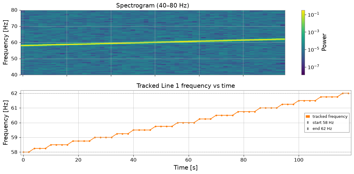
Detection rate: 60/60 frames (100 %)
Freq range: 58.00 – 62.00 Hz

5. Multi-Line Tracking

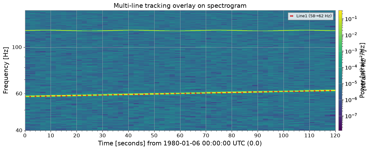
Run one tracker per seed frequency and overlay results on the spectrogram for visual verification.

import warnings

with warnings.catch_warnings():

    # ── Track both lines simultaneously ──────────────────────────────────────────
    SEEDS = {
    "Line1 (58→62 Hz)": 58.5,
    "Line2 (120 Hz)":   120.0,
    }

    tracks = {name: track_line(spec, seed, max_jump=2.5)
    for name, seed in SEEDS.items()}

    # ── Overlay on spectrogram ────────────────────────────────────────────────────
    colors = ["tab:red", "tab:cyan"]

    _plt_sp = spec.plot(norm="log", figsize=(12, 5))
    ax = _plt_sp.gca()
    fig = _plt_sp.figure
    ax.set_ylim(40, 150)
    _plt_sp.colorbar(label="Power [strain²/Hz]")

    for (name, trk), color in zip(tracks.items(), colors):
        mask = ~np.isnan(trk)
        ax.plot(times[mask], trk[mask], "o", ms=3, color=color,
        label=name, alpha=0.85)

        ax.set_title("Multi-line tracking overlay on spectrogram")
        ax.legend(loc="upper right", fontsize=9)
        with warnings.catch_warnings():
            warnings.filterwarnings("ignore", message="This figure includes Axes that are not compatible with tight_layout")
        plt.tight_layout()
        plt.show()

<Figure size 1200x400 with 0 Axes>

6. Frequency Drift Visualisation

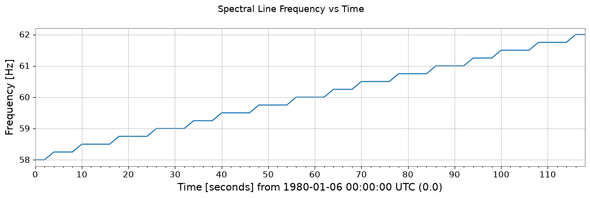
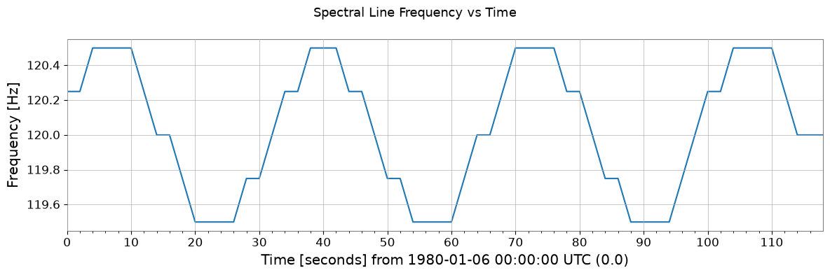
Wrap each track in a TimeSeries to plot frequency evolution and compute basic drift statistics.

import warnings

with warnings.catch_warnings():

    # ── Build TimeSeries from tracking results and plot frequency evolution ────────
    fig, axes = plt.subplots(len(tracks), 1, figsize=(12, 5), sharex=True)

    for ax, (name, trk) in zip(axes, tracks.items()):
        mask    = ~np.isnan(trk)
        t_valid = times[mask]
        f_valid = trk[mask]

        ts_freq = TimeSeries(f_valid, times=t_valid, name=name, unit="Hz")
        ts_freq.plot(ax=ax)
        ax.set_ylabel("Frequency [Hz]")
        ax.set_title(name)

        axes[-1].set_xlabel("Time [s]")
        plt.suptitle("Spectral Line Frequency vs Time", fontsize=13)
        with warnings.catch_warnings():
            warnings.filterwarnings("ignore", message="This figure includes Axes that are not compatible with tight_layout")
        plt.tight_layout()
        plt.show()

        # ── Drift statistics ─────────────────────────────────────────────────────────
        print(f"{'Line':<25} {'min [Hz]':>10} {'max [Hz]':>10} {'drift [Hz]':>12}")
        print("-" * 60)
        for name, trk in tracks.items():
            lo, hi = np.nanmin(trk), np.nanmax(trk)
            print(f"{name:<25} {lo:>10.3f} {hi:>10.3f} {hi - lo:>12.3f}")

Line                        min [Hz]   max [Hz]   drift [Hz]
------------------------------------------------------------
Line1 (58→62 Hz)              58.000     62.000        4.000
Line2 (120 Hz)               119.500    120.500        1.000

Line                        min [Hz]   max [Hz]   drift [Hz]
------------------------------------------------------------
Line1 (58→62 Hz)              58.000     62.000        4.000
Line2 (120 Hz)               119.500    120.500        1.000

print("=" * 60)
print("Peak / Line Tracking — Key Steps")
print("-" * 60)
steps = [
    ("1. spectrogram2()",       "Compute time-frequency power map"),
    ("2. sp_find_peaks(row)",   "Detect peaks in each time frame"),
    ("3. nearest-neighbour",    "Connect peaks across frames by min-dist"),
    ("4. NaN on miss",          "Mark undetected frames as NaN"),
    ("5. TimeSeries(track)",    "Build frequency-vs-time TimeSeries"),
]
for s, d in steps:
    print(f"  {s:<25} {d}")
print("=" * 60)

============================================================
Peak / Line Tracking — Key Steps
------------------------------------------------------------
  1. spectrogram2()         Compute time-frequency power map
  2. sp_find_peaks(row)     Detect peaks in each time frame
  3. nearest-neighbour      Connect peaks across frames by min-dist
  4. NaN on miss            Mark undetected frames as NaN
  5. TimeSeries(track)      Build frequency-vs-time TimeSeries
============================================================