
Coupling Analysis: Multi-Channel Coupling#
This tutorial demonstrates the Coupling Function (CF) analysis workflow using gwexpy.analysis.CouplingFunctionAnalysis.
What is a Coupling Function?#
A coupling function quantifies how much a witness (environmental) sensor’s noise couples into a target (sensitive) channel. It is defined as:
where \(P_{\rm inj}\) and \(P_{\rm bkg}\) are the power spectral densities during injection and background periods.
Typical application: PEM (Physical Environment Monitor) injection analysis in gravitational-wave detectors.
Legacy migration note:
If your legacy code manually computed PSDs, divided them, and applied custom thresholds via scipy, this workflow replaces all of that.
See the GWexpy for GWpy Users guide and GWpy Difference API Index for migration guidance.
Note — SigmaThreshold statistical validity: When the number of averaged segments
n_avgis below 10, the Gaussian approximation of the χ²(2K) distribution becomes less accurate. AUserWarningwill be raised in this case. Consider usingPercentileThresholdfor short data segments.
import warnings


import matplotlib.pyplot as plt
import numpy as np
from astropy import units as u

from gwexpy.analysis.coupling import (
    CouplingFunctionAnalysis,
    RatioThreshold,
    SigmaThreshold,
)
from gwexpy.timeseries import TimeSeries, TimeSeriesDict
1. Prepare Synthetic Injection / Background Data#
We simulate:
A witness channel (environmental sensor): seismic or acoustic
Two target channels (sensitive instruments): one strongly coupled, one weakly coupled
The injection adds a coherent tone to the witness. The targets respond proportionally to the coupling strength.
rng = np.random.default_rng(0)

fs   = 512     # sample rate [Hz]
T    = 32.0    # duration [s]
n    = int(fs * T)
t    = np.arange(n) / fs
dt   = (1 / fs) * u.s

# Frequency bins for injected tones
f_inj1 = 12.5   # Hz
f_inj2 = 25.0   # Hz

# Noise floor
noise_level = 0.1

# --- Background data (no injection) ---
wit_bkg  = rng.normal(0, noise_level, n)
tgt1_bkg = rng.normal(0, noise_level, n)
tgt2_bkg = rng.normal(0, noise_level, n)

# --- Injection data: excite the witness with tones ---
inj_signal = 5.0 * np.sin(2 * np.pi * f_inj1 * t) + 3.0 * np.sin(2 * np.pi * f_inj2 * t)

wit_inj  = inj_signal + rng.normal(0, noise_level, n)

# Target 1: strong coupling (CF ≈ 0.4 at f_inj1, 0.3 at f_inj2)
cf_true1 = 0.4
tgt1_inj = cf_true1 * inj_signal + rng.normal(0, noise_level, n)

# Target 2: weak coupling (CF ≈ 0.05)
cf_true2 = 0.05
tgt2_inj = cf_true2 * inj_signal + rng.normal(0, noise_level, n)

# Wrap in TimeSeries
def make_ts(data, name, unit=u.ct):
    return TimeSeries(data, dt=dt, t0=0*u.s, unit=unit, name=name)

# Background dict
data_bkg = TimeSeriesDict({
    "ACC:FLOOR_X":  make_ts(wit_bkg,  "ACC:FLOOR_X",  u.m / u.s**2),
    "GW:DARM":      make_ts(tgt1_bkg, "GW:DARM",      u.m),
    "GW:AUX":       make_ts(tgt2_bkg, "GW:AUX",       u.m),
})

# Injection dict
data_inj = TimeSeriesDict({
    "ACC:FLOOR_X":  make_ts(wit_inj,  "ACC:FLOOR_X",  u.m / u.s**2),
    "GW:DARM":      make_ts(tgt1_inj, "GW:DARM",      u.m),
    "GW:AUX":       make_ts(tgt2_inj, "GW:AUX",       u.m),
})

print("Background channels:", list(data_bkg.keys()))
print("Injection channels: ", list(data_inj.keys()))
Background channels: ['ACC:FLOOR_X', 'GW:DARM', 'GW:AUX']
Injection channels:  ['ACC:FLOOR_X', 'GW:DARM', 'GW:AUX']
2. Run Coupling Function Analysis#
CouplingFunctionAnalysis.compute() takes the injection and background TimeSeriesDict, and the name of the witness channel.
cfa = CouplingFunctionAnalysis()

results = cfa.compute(
    data_inj=data_inj,
    data_bkg=data_bkg,
    fftlength=4.0,          # 4-second FFT segments
    overlap=0.5,             # 50% overlap
    witness="ACC:FLOOR_X",  # the environmental sensor
    threshold_witness=RatioThreshold(ratio=10.0),   # witness must show 10× excess
    threshold_target=RatioThreshold(ratio=2.0),     # target must show 2× excess
)

print("Results computed for:", list(results.keys()))
Results computed for: ['GW:DARM', 'GW:AUX']
3. Inspect Results#
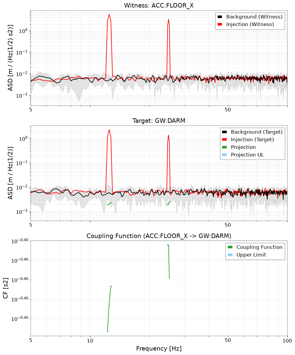
Each result is a CouplingResult containing the coupling function, upper limit, and diagnostic PSDs.
# Strong coupling channel (GW:DARM)
res_darm = results["GW:DARM"]

print("CF valid bins:", res_darm.valid_mask.sum())
print("CF at f_inj1 bin:", end=" ")

freqs = res_darm.cf.frequencies.value
idx1 = np.argmin(np.abs(freqs - f_inj1))
idx2 = np.argmin(np.abs(freqs - f_inj2))
print(f"{res_darm.cf.value[idx1]:.3f} (expected ~{cf_true1})")
print(f"CF at f_inj2 bin: {res_darm.cf.value[idx2]:.3f} (expected ~{cf_true1})")

# Simple CF plot
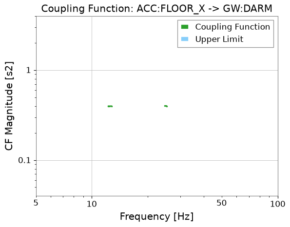
res_darm.plot_cf(xlim=(5, 100));
CF valid bins: 6
CF at f_inj1 bin: 0.400 (expected ~0.4)
CF at f_inj2 bin: 0.401 (expected ~0.4)
# Full diagnostic plot: Witness ASD | Target ASD | CF
res_darm.plot(xlim=(5, 100));
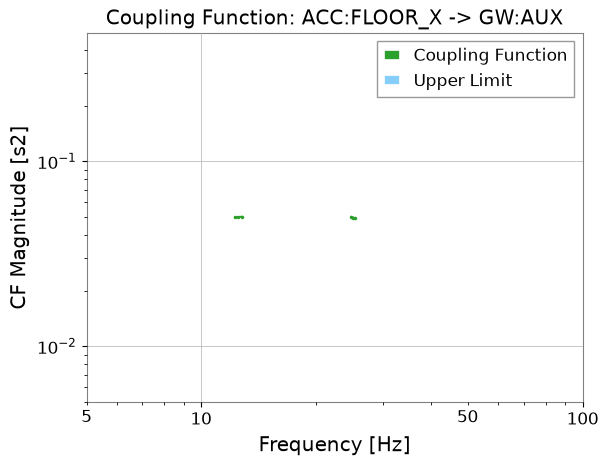
# Weak coupling channel (GW:AUX)
res_aux = results["GW:AUX"]
print("GW:AUX valid CF bins:", res_aux.valid_mask.sum())
res_aux.plot_cf(xlim=(5, 100));
GW:AUX valid CF bins: 6
import warnings
4. Threshold Strategies#
gwexpy provides three built-in threshold strategies:
Strategy |
Description |
Best for |
|---|---|---|
|
\(P_{\rm inj} > r \cdot P_{\rm bkg}\) |
Fast screening, physical reasoning |
|
Gaussian significance test |
Stationary, Gaussian backgrounds |
|
Empirical distribution |
Non-Gaussian, glitchy backgrounds |
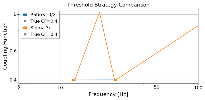
import warnings

with warnings.catch_warnings():

    # Compare threshold strategies
    n_avg = T / 4.0  # approximate averaging count for 4-second FFT

    strategies = {
    "Ratio×10/2":   (RatioThreshold(10.0), RatioThreshold(2.0)),
    "Sigma 3σ":      (SigmaThreshold(3.0),  SigmaThreshold(2.0)),
    }

    fig, ax = plt.subplots(figsize=(8, 4))

    for label, (thr_w, thr_t) in strategies.items():
        res = cfa.compute(
        data_inj=data_inj,
        data_bkg=data_bkg,
        fftlength=4.0,
        overlap=0.5,
        witness="ACC:FLOOR_X",
        threshold_witness=thr_w,
        threshold_target=thr_t,
        )
        cf = res["GW:DARM"].cf
        valid = ~np.isnan(cf.value)
        ax.plot(cf.frequencies.value[valid], cf.value[valid], marker=".", label=label)

        ax.axhline(cf_true1, color="gray", linestyle="--", label=f"True CF={cf_true1}")
        ax.set_xscale("log")
        ax.set_yscale("log")
        ax.set_xlim(5, 100)
        ax.set_xlabel("Frequency [Hz]")
        ax.set_ylabel("Coupling Function")
        ax.set_title("Threshold Strategy Comparison")
        ax.legend()
        plt.tight_layout()
/tmp/ipykernel_4849/3140365492.py:16: UserWarning: SigmaThreshold: n_avg=9.0 < 10. Gaussian approximation may be inaccurate for χ²(2K) with K < 10. Consider using PercentileThreshold for more robust results.
  res = cfa.compute(
/home/runner/work/gwexpy/gwexpy/gwexpy/analysis/coupling.py:833: UserWarning: SigmaThreshold: n_avg=9.0 < 10. Gaussian approximation may be inaccurate for χ²(2K) with K < 10. Consider using PercentileThreshold for more robust results.
  res = _process_single_target(
5. Frequency Range Restriction#
Use frange to restrict the coupling function evaluation to a specific frequency band.
results_band = cfa.compute(
    data_inj=data_inj,
    data_bkg=data_bkg,
    fftlength=4.0,
    overlap=0.5,
    witness="ACC:FLOOR_X",
    frange=(10.0, 50.0),   # only evaluate 10–50 Hz
)

cf_band = results_band["GW:DARM"].cf
valid_band = ~np.isnan(cf_band.value)
print(f"Valid CF bins in 10–50 Hz: {valid_band.sum()}")
results_band["GW:DARM"].plot_cf(xlim=(5, 100));
Valid CF bins in 10–50 Hz: 6
6. Upper Limits#
At frequencies where the witness is excited but the target shows no measurable excess, gwexpy computes an upper limit on the coupling function.
This is useful for setting constraints even when the coupling is below the noise floor.
# Upper limit is automatically computed in cf_ul attribute
res_darm = results["GW:DARM"]

cf_ul = res_darm.cf_ul
ul_valid = ~np.isnan(cf_ul.value)
print(f"Upper limit bins: {ul_valid.sum()}")

# The full diagnostic plot includes both CF and upper limit
res_darm.plot_cf(xlim=(5, 100));
Upper limit bins: 0
Summary#
from gwexpy.analysis.coupling import CouplingFunctionAnalysis, RatioThreshold

cfa = CouplingFunctionAnalysis()
results = cfa.compute(
    data_inj=data_inj,        # TimeSeriesDict with injection data
    data_bkg=data_bkg,        # TimeSeriesDict with background data
    fftlength=4.0,
    witness="ACC:FLOOR_X",
    threshold_witness=RatioThreshold(25.0),
    threshold_target=RatioThreshold(4.0),
)

# Access result for one target
res = results["GW:DARM"]
res.plot()         # diagnostic 3-panel plot
res.cf             # FrequencySeries: coupling function values
res.cf_ul          # FrequencySeries: upper limits
See also: