Case navigation:
Back to the canonical gallery: Case Studies
Related reference surfaces: Reference Index, API: Frequency Series
Neighboring featured workflows: Noise Budgeting, Active Damping
Tutorial: Transfer Function Measurement#
This tutorial demonstrates how to use gwexpy to estimate the transfer function of a system from measured data,
fit a physical model to the transfer function, and identify system parameters.
Scenario: We inject white noise into a mechanical vibration system (or electrical circuit) and measure its response. From this input-output data, we will determine the system’s resonance frequency \(f_0\) and quality factor \(Q\).
Workflow:
Data generation: Simulate an input signal (white noise) and the system output (resonant system response + measurement noise).
Transfer function estimation: Calculate the transfer function and coherence from the input-output time series data and plot the Bode plot.
Model fitting: Fit a theoretical model (such as a Lorentzian function) to the estimated transfer function to extract system parameters.
import warnings


import matplotlib.pyplot as plt
import numpy as np
np.random.seed(42)
from scipy import signal

from gwexpy import TimeSeries
from gwexpy.plot import Plot
1. Generating Experimental Data (Simulation)#
We will conduct a virtual experiment.
System: Second-order resonant system (harmonic oscillator)
Resonance frequency \(f_0 = 300\) Hz
Quality factor \(Q = 50\)
Input: White noise
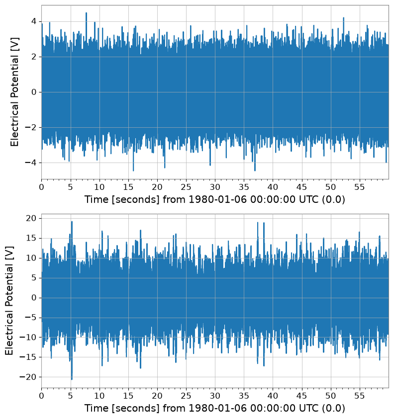
Measurement: Sampling frequency 2048 Hz, duration 60 seconds
The output signal will also include measurement noise.
# --- Parameter Settings: choose a resonator whose f0 and Q mimic a narrow mechanical mode worth identifying from measured data. ---
fs = 2048.0  # Sampling frequency [Hz]
duration = 60.0  # Duration [s]
f0_true = 300.0  # True resonance frequency [Hz]
Q_true = 50.0  # True quality factor

# --- Time axis and input signal: broadband drive excites the plant across frequency so the resonance can be measured in one experiment. ---
t = np.linspace(0, duration, int(duration * fs), endpoint=False)
input_data = np.random.normal(0, 1, size=len(t))  # Broadband excitation approximates a swept identification drive without privileging one frequency.

# --- Physical System Simulation (using scipy.signal): this second-order plant stands in for a suspension or actuator resonance. ---
# H(s) uses f0 for the modal frequency and Q for damping width, so fitting them back out tests whether the measurement preserves the true mode shape.
w0 = 2 * np.pi * f0_true
num = [w0**2]
den = [1, w0 / Q_true, w0**2]
system = signal.TransferFunction(num, den)

# Simulate the time response to the broadband drive so transfer estimation sees the same finite-duration effects as a real measurement.
_, output_clean, _ = signal.lsim(system, U=input_data, T=t)

# --- Add measurement noise: coherence later tells us whether this readout noise is low enough to trust the estimated transfer function. ---
# Treat this as sensor/readout noise, which degrades phase and gain estimates where the plant response is weak.
measurement_noise = np.random.normal(0, 0.1, size=len(t))
output_data = output_clean + measurement_noise

# --- Wrap the drive and response as TimeSeries so the same workflow applies to experimental channels. ---
ts_input = TimeSeries(input_data, t0=0, sample_rate=fs, name="Input", unit="V")
ts_output = TimeSeries(output_data, t0=0, sample_rate=fs, name="Output", unit="V")

print("Input data shape:", ts_input.shape)
print("Output data shape:", ts_output.shape)
Plot(ts_input, ts_output, separate=True);
Input data shape: (122880,)
Output data shape: (122880,)
2. Transfer Function Estimation#
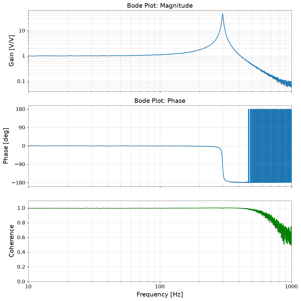
From the input-output time series data ts_input and ts_output, we estimate the frequency response function (transfer function).
We use the transfer_function method of gwexpy.
We also calculate the coherence to assess the reliability of the measurement. Frequency bands where the coherence is close to 1 indicate that the input-output relationship is linear and the influence of noise is small.
# FFT settings: average 2-second segments so random measurement noise is reduced without washing out the 300 Hz resonance.
fftlength = 2.0  # FFT every 2 seconds and average

# Estimate Output/Input so the plant response appears directly in gain and phase.
tf = ts_input.transfer_function(ts_output, fftlength=fftlength)

# Coherence is the confidence check: low coherence means the response is noise dominated and the transfer estimate should not be over-interpreted.
coh = ts_input.coherence(ts_output, fftlength=fftlength) ** 0.5

# --- Plot Bode magnitude, phase, and coherence together so trustworthiness and fitted physics can be read on the same axis. ---
fig, axes = plt.subplots(3, 1, figsize=(10, 10), sharex=True)

# Magnitude
ax = axes[0]
ax.loglog(tf.abs(), label="Measured TF")
ax.set_ylabel("Gain [V/V]")
ax.set_title("Bode Plot: Magnitude")
ax.grid(True, which="both", alpha=0.5)

# Phase
ax = axes[1]
ax.plot(tf.degree(), label="Measured Phase")
ax.set_ylabel("Phase [deg]")
ax.set_title("Bode Plot: Phase")
ax.set_yticks(np.arange(-180, 181, 90))
ax.grid(True, which="both", alpha=0.5)

# Coherence
ax = axes[2]
ax.plot(coh, color="green", label="Coherence")
ax.set_ylabel("Coherence")
ax.set_xlabel("Frequency [Hz]")
ax.set_ylim(0, 1.1)
ax.set_xlim(10, 1000)
ax.grid(True, which="both", alpha=0.5)

plt.tight_layout()
plt.show()
3. Model Fitting#
We fit a theoretical model to the obtained transfer function (especially around the resonance). Here, we define a transfer function model for a harmonic oscillator and use least-squares fitting to determine the parameters (\(A, f_0, Q\)).
Model equation (including gain \(A\)): $\( H(f) = A \cdot \frac{f_0^2}{f_0^2 - f^2 + i (f f_0 / Q)} \)$
# --- Define a resonator model whose parameters map back to measurable plant physics. ---
def resonator_model(f, amp, f0, Q):
    # f: frequency array in Hz where the measured plant response is sampled.
    # amp scales the actuator/sensor gain, f0 is the modal resonance, and Q controls how sharply energy stays trapped near that mode.

    # Use the complex response so the fit respects both magnitude and phase, not just the height of the peak.
    numerator = amp * (f0**2)
    denominator = (f0**2) - (f**2) + 1j * (f * f0 / Q)
    return numerator / denominator


# --- Fit only the resonance-dominated band so broadband tails do not bias the modal parameters. ---
# Fitting the full band would force one second-order model to explain off-resonance structure it was never meant to capture,
# so we isolate 100-500 Hz where the identified mode dominates the response.
tf_crop = tf.crop(100, 500)

# Seed f0 near the visible peak so the optimizer lands on the physical resonance instead of a spurious local minimum.
# The initial guess is intentionally close to the observed resonance around 300 Hz.
p0 = {"amp": 1.0, "f0": 300.0, "Q": 10.0}

# Fit the complex transfer function in this narrowed band.
# .fit() uses both real and imaginary parts, which preserves phase information needed to recover damping consistently.
result = tf_crop.fit(resonator_model, p0=p0)

print(result)
┌─────────────────────────────────────────────────────────────────────────┐
│                                Migrad                                   │
├──────────────────────────────────┬──────────────────────────────────────┤
│ FCN = 6.348 (χ²/ndof = 0.0)      │              Nfcn = 118              │
│ EDM = 3.95e-06 (Goal: 0.0002)    │                                      │
├──────────────────────────────────┼──────────────────────────────────────┤
│          Valid Minimum           │   Below EDM threshold (goal x 10)    │
├──────────────────────────────────┼──────────────────────────────────────┤
│      No parameters at limit      │           Below call limit           │
├──────────────────────────────────┼──────────────────────────────────────┤
│             Hesse ok             │         Covariance accurate          │
└──────────────────────────────────┴──────────────────────────────────────┘
┌───┬──────┬───────────┬───────────┬────────────┬────────────┬─────────┬─────────┬───────┐
│   │ Name │   Value   │ Hesse Err │ Minos Err- │ Minos Err+ │ Limit-  │ Limit+  │ Fixed │
├───┼──────┼───────────┼───────────┼────────────┼────────────┼─────────┼─────────┼───────┤
│ 0 │ amp  │   0.935   │   0.007   │            │            │         │         │       │
│ 1 │ f0   │  299.996  │   0.021   │            │            │         │         │       │
│ 2 │ Q    │   49.4    │    0.5    │            │            │         │         │       │
└───┴──────┴───────────┴───────────┴────────────┴────────────┴─────────┴─────────┴───────┘
┌─────┬────────────────────────────┐
│     │      amp       f0        Q │
├─────┼────────────────────────────┤
│ amp │ 4.34e-05       -0 -2.28e-3 │
│  f0 │       -0 0.000456  -0.1e-3 │
│   Q │ -2.28e-3  -0.1e-3     0.24 │
└─────┴────────────────────────────┘
4. Verification of Results#
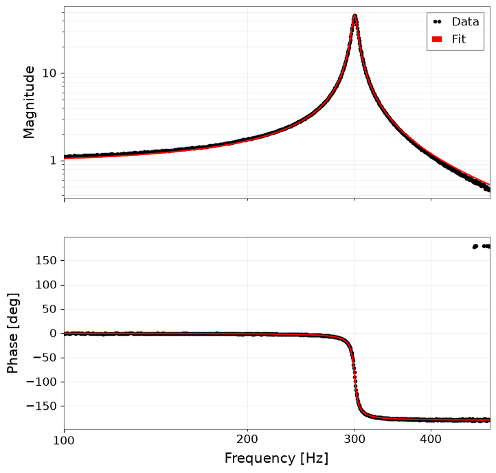
We verify the fitting results numerically and plot them overlaid on the measured data.
The FitResult.plot() method automatically generates a Bode plot (magnitude and phase) for complex data.
# --- Report the recovered modal parameters so they can be compared with the known plant values. ---
print("--- Estimated Parameters ---")
print(f"Resonance Frequency (f0): {result.params['f0']:.4f} Hz (True: {f0_true})")
print(f"Quality Factor (Q):       {result.params['Q']:.4f}      (True: {Q_true})")
print(f"Gain (Amp):               {result.params['amp']:.4f}")

# --- Plot the fitted response to confirm that both the peak height and phase rotation are captured. ---
# result.plot() returns magnitude and phase axes because both observables are needed to judge whether the modal model is credible.
axes = result.plot()
plt.show()
--- Estimated Parameters ---
Resonance Frequency (f0): 299.9962 Hz (True: 300.0)
Quality Factor (Q):       49.3695      (True: 50.0)
Gain (Amp):               0.9345