Development documentation · 0.2.3 30c2f8ba · Intro examples tested with 0.2.3 · Version details · Known limitations

Histogram: Basics

This tutorial introduces gwexpy.histogram.Histogram and demonstrates:

• Creating histograms (from totals, from events using .fill())

• Visualization (counts and density)

• Basic statistics (mean, median, variance, quantiles)

• Rebinning with covariance propagation

• Integration with error propagation

• Serialization (HDF5 and JSON)

• ROOT interoperability (optional; handled with try/except)

Run this notebook in the gwexpy conda environment so that all dependencies are available.

import warnings


# Environment check
import sys

import matplotlib.pyplot as plt
import numpy as np
from astropy import units as u

from gwexpy.histogram import Histogram

print('python', sys.version.splitlines()[0])
print('numpy', np.__version__)
print('astropy', u.__version__ if hasattr(u, '__version__') else 'unknown')

python 3.11.16 (main, Sep  2 2026, 23:39:52) [GCC 15.3.0]
numpy 2.4.6
astropy unknown

1. Creating Histograms

Two common ways to create a Histogram:

1. Directly from bin totals and edges

2. From raw events using .fill() (supports astropy.units.Quantity weights)

# 1.1 Direct construction from totals
edges = np.array([0.0, 1.0, 2.0, 4.0])
values = np.array([10.0, 25.0, 15.0])  # bin totals
h = Histogram(values=values, edges=edges, unit='count')
h

<Histogram (nbins=3, unit=ct)>

# 1.2 Creating from events with weights (Quantity)
rng = np.random.RandomState(42)
events = np.concatenate([
    rng.normal(0.5, 0.1, size=50),
    rng.normal(1.6, 0.2, size=120),
    rng.normal(3.0, 0.3, size=80)
])
weights = u.Quantity(rng.uniform(0.5, 2.0, size=events.size), unit='count')
h2 = Histogram(values=np.zeros(len(edges)-1), edges=edges, unit='count').fill(events, weights=weights)
h2

<Histogram (nbins=3, unit=ct)>

2. Visualization

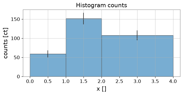
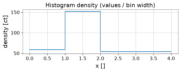
Plot bin totals (with errorbars if available) and density (value / bin width).

# Plot counts with errorbars
fig, ax = plt.subplots(figsize=(7,3))
centers = h2.bin_centers.value
widths = h2.bin_widths.value
counts = h2.values.value
errs = (h2.errors.value if h2.errors is not None else None)
ax.bar(centers, counts, width=widths, align='center', edgecolor='k', alpha=0.6)
if errs is not None:
    ax.errorbar(centers, counts, yerr=errs, fmt='none', ecolor='k')
ax.set_xlabel(f"x [{h2.xunit}]")
ax.set_ylabel(f"counts [{h2.unit}]")
ax.set_title('Histogram counts')
plt.show()

# Density plot (values / bin width)
density = h2.to_density()
fig, ax = plt.subplots(figsize=(7,2))
ax.step(h2.edges.value, np.append(density.value, density.value[-1]), where='post')
ax.set_xlabel(f"x [{h2.xunit}]")
ax.set_ylabel(f"density [{density.unit}]")
ax.set_title('Histogram density (values / bin width)')
plt.show()

3. Basic statistics

Compute mean, median, variance and quantiles. quantile() is robust to flat bins.

print('mean:', h2.mean())
print('median:', h2.median())
print('variance:', h2.var())
print('std:', h2.std())
print('quantile(0.25):', h2.quantile(0.25))

mean: 1.8213054429831148
median: 1.6599075323583463
variance: 0.8432605001074853
std: 0.918292164894967
quantile(0.25): 1.1348114645471883

4. Rebinning

Demonstrate rebinning to non-uniform bins and verify totals are conserved and covariance is propagated.

new_edges = np.array([0.0, 1.5, 4.0])
h_reb = h2.rebin(new_edges)
print('sum original:', h2.values.sum())
print('sum rebinned:', h_reb.values.sum())
print('cov present original:', h2.cov is not None)
print('cov shape rebinned:', h_reb.cov.shape if h_reb.cov is not None else None)

sum original: 318.85040365900875 ct
sum rebinned: 318.85040365900875 ct
cov present original: False
cov shape rebinned: None

5. Integration with error propagation

Integrate over a partial interval (handles partial bin overlap) and show the propagated error.

I = h2.integral(0.7, 2.2)
I_val, I_err = h2.integral(0.7, 2.2, return_error=True)
print('Integral (no error):', I)
print('Integral with error:', I_val, I_err)

Integral (no error): 180.3597019890495 ct
Integral with error: 180.3597019890495 ct 15.17057636890394 ct

6. Serialization (HDF5 and JSON)

Show HDF5 write/read and a JSON-friendly dict for light-weight exchange.

# HDF5 roundtrip
import tempfile
from pathlib import Path

hist_path = Path(tempfile.gettempdir()) / 'gwexpy_example_hist.h5'
h2.write(hist_path, format='hdf5', path='hist1')
h_loaded = Histogram.read(hist_path, format='hdf5', path='hist1')
print('HDF5 roundtrip equal (values):', np.allclose(h2.values.value, h_loaded.values.value))

HDF5 roundtrip equal (values): True

import json


def hist_to_json_dict(h):
    def get_val(x):
        return x.value if hasattr(x, 'value') else x
    return {
        'values': h.values.value.tolist(),
        'edges': h.edges.value.tolist(),
        'unit': str(h.unit),
        'xunit': str(h.xunit),
        'cov': (h.cov.value.tolist() if h.cov is not None else None),
        'sumw2': (h.sumw2.value.tolist() if h.sumw2 is not None else None),
        'underflow': float(get_val(getattr(h, 'underflow', 0.0))),
        'overflow': float(get_val(getattr(h, 'overflow', 0.0))),
    }
def hist_from_json_dict(d):
    kwargs = {}
    if d.get('cov') is not None:
        kwargs['cov'] = np.array(d['cov'])
    if d.get('sumw2') is not None:
        kwargs['sumw2'] = np.array(d['sumw2'])
    if d.get('underflow') is not None:
        kwargs['underflow'] = d['underflow']
    if d.get('overflow') is not None:
        kwargs['overflow'] = d['overflow']
    return Histogram(values=np.array(d['values']), edges=np.array(d['edges']), unit=d['unit'], xunit=d['xunit'], **kwargs)

j = hist_to_json_dict(h2)
open('hist.json','w').write(json.dumps(j, indent=2))
h_j = hist_from_json_dict(json.loads(open('hist.json').read()))
print('JSON roundtrip (values):', np.allclose(h2.values.value, h_j.values.value))

JSON roundtrip (values): True

7. ROOT interoperability (optional)

PyROOT may not be present in all environments. Use try/except to handle absence gracefully.

try:
    th1 = h2.to_th1d()
    print("TH1D created:", th1.GetName(), "nbins:", th1.GetNbinsX())
    print("ROOT underflow:", th1.GetBinContent(0))
    h_from_root = Histogram.from_root(th1)
    np.testing.assert_allclose(h_from_root.value, h2.value)
    print("Back to Histogram:", h_from_root)
except ImportError as exc:
    print("Optional ROOT example skipped:", exc)

Optional ROOT example skipped: The 'ROOT' package is required for this feature but is not installed. You can install it via 'pip install ROOT'.

8. Exercises

1. Generate a 1D mixture of Gaussians and verify rebin totals are preserved.

2. Create weighted events where weights are Quantity and verify sumw2 updates as sum(w^2).

3. Save a histogram to HDF5 and JSON, and load it back in a separate Python process to check equality.

Summary

• Histogram stores bin totals and propagates covariance under linear transforms (rebin).

• fill() supports Quantity weights and updates sumw2/cov appropriately.

• Use HDF5 for lossless IO; JSON for light-weight exchange.

• For very large nbins, consider sparse/low-rank covariance representations.