Development documentation · 0.2.3 30c2f8ba · Intro examples tested with 0.2.3 · Version details · Known limitations

SpectrogramMatrix: Matrix Basics

This notebook introduces the basic usage of the SpectrogramMatrix class in gwexpy.

SpectrogramMatrix is a class designed to efficiently handle multiple gwpy.spectrogram.Spectrogram objects as a 3-dimensional matrix (Batch, Time, Frequency). It inherits from numpy.ndarray, enabling fast numerical computation and seamless integration with PyTorch/CuPy.

import warnings


import astropy.units as u
import matplotlib.pyplot as plt
import numpy as np

from gwexpy.timeseries import TimeSeriesMatrix

# Fix random seed
np.random.seed(42)

1. Data Preparation

rng = np.random.default_rng(0)

# Sample configuration
n = 512
dt = (1 / 128) * u.s
t0 = 0 * u.s

t = (np.arange(n) * dt).to_value(u.s)

tone50 = np.sin(2 * np.pi * 50 * t)
tone20 = np.sin(2 * np.pi * 20 * t + 0.3)

data = np.empty((2, 2, n), dtype=float)
data[0, 0] = 0.5 * tone50 + 0.05 * rng.normal(size=n)
data[0, 1] = 0.5 * tone20 + 0.05 * rng.normal(size=n)
data[1, 0] = 0.3 * tone50 + 0.3 * tone20 + 0.05 * rng.normal(size=n)
data[1, 1] = 0.2 * tone50 - 0.4 * tone20 + 0.05 * rng.normal(size=n)

units = np.full((2, 2), u.V)
names = [["ch00", "ch01"], ["ch10", "ch11"]]
channels = [["X:A", "X:B"], ["Y:A", "Y:B"]]

tsm = TimeSeriesMatrix(
    data,
    dt=dt,
    t0=t0,
    units=units,
    names=names,
    channels=channels,
    rows={"r0": {"name": "row0"}, "r1": {"name": "row1"}},
    cols={"c0": {"name": "col0"}, "c1": {"name": "col1"}},
    name="demo",
)

display(tsm)
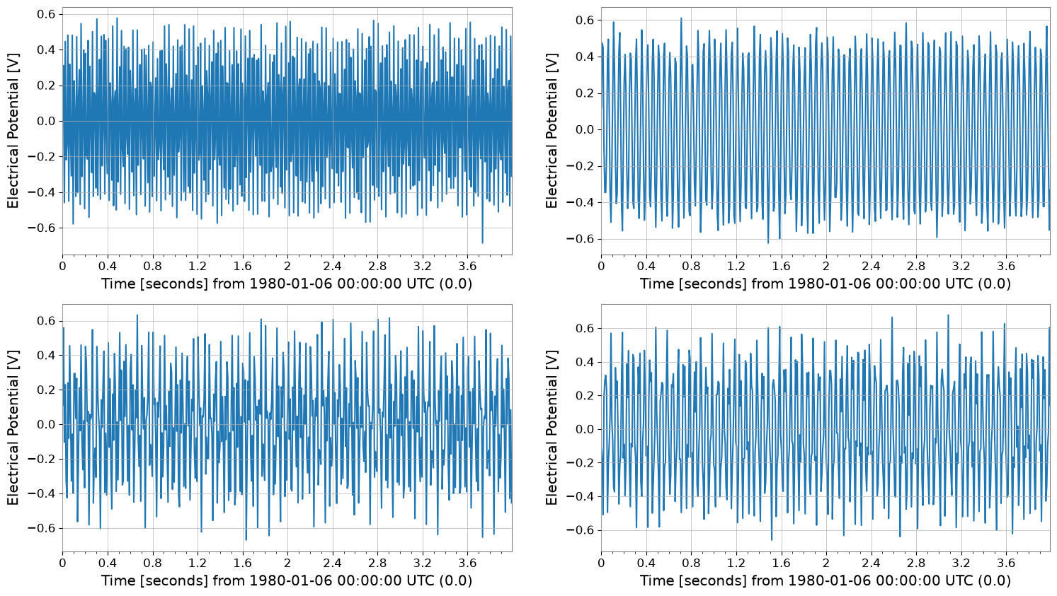
tsm.plot()
plt.show()

SeriesMatrix: shape=(2, 2, 512), name='demo'

• epoch: 0.0 s
• x0: 0.0 s, dx: 0.0078125 s, N_samples: 512
• xunit: s

Row Metadata

	name	channel	unit
key
r0	row0
r1	row1

Column Metadata

	name	channel	unit
key
c0	col0
c1	col1

Element Metadata

	unit	name	channel	row	col
0	V	ch00	X:A	0	0
1	V	ch01	X:B	0	1
2	V	ch10	Y:A	1	0
3	V	ch11	Y:B	1	1

2. Creating a SpectrogramMatrix

Using the to_matrix() method of SpectrogramList, all spectrograms are stacked into a single SpectrogramMatrix. This yields a 3-dimensional array with shape (N, Time, Frequency).

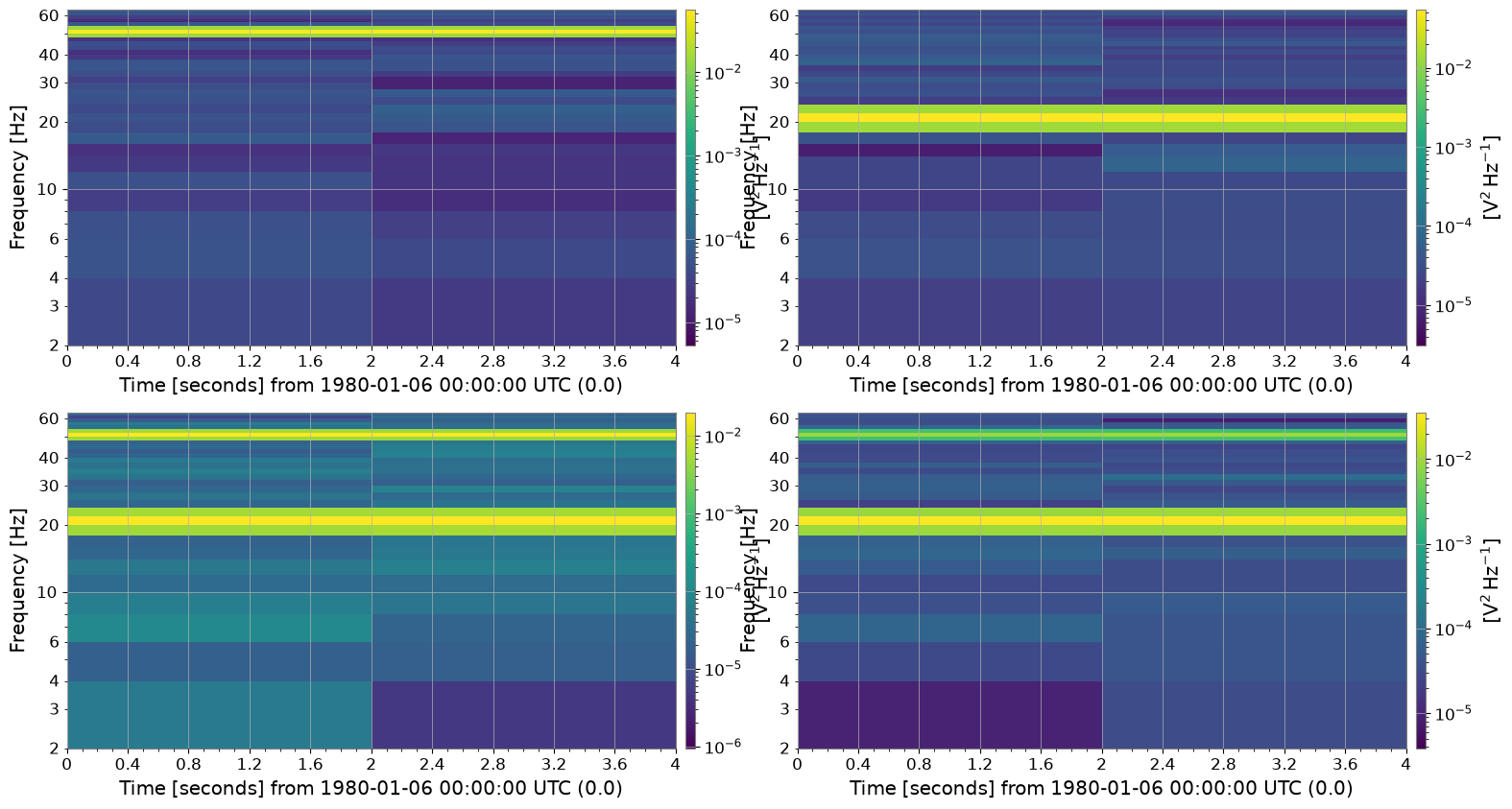
spec_matrix = tsm.spectrogram(2, fftlength=0.5, overlap=0.25)

print("Type:", type(spec_matrix))
print("Shape:", spec_matrix.shape)  # (Batch, Time, Freq)
spec_matrix.plot();

Type: <class 'gwexpy.spectrogram.matrix.SpectrogramMatrix'>
Shape: (2, 2, 2, 33)

Accessing Attributes

SpectrogramMatrix preserves information about the time and frequency axes from the original spectrograms.

print("Time axis (first 5):", spec_matrix.times[:5])
print("Freq axis (first 5):", spec_matrix.frequencies[:5])
print("Unit:", spec_matrix.unit)

Time axis (first 5): [0. 2.] s
Freq axis (first 5): [0. 2. 4. 6. 8.] Hz
Unit: V2 / Hz

3. Numerical Computation and Statistics

Since SpectrogramMatrix is a subclass of numpy.ndarray, NumPy functions can be applied directly. Methods like mean() are also available.

For example, let’s calculate the average spectrogram across all channels (batch dimension).

# Take the mean along axis=0 (Batch axis)
mean_spectrogram_data = spec_matrix.mean(axis=0)

print("Mean Data Shape:", mean_spectrogram_data.shape)
# The result is a 2D array of shape (Time, Freq)

Mean Data Shape: (2, 2, 33)

4. Plotting

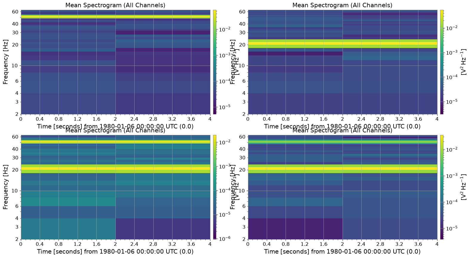
Use the plot() method to visualize the data. When calling plot() on 3-dimensional data (Batch, Time, Freq), by default the mean across the batch dimension is plotted. This is useful for examining the average characteristics across multiple events.

plot = spec_matrix.plot(title="Mean Spectrogram (All Channels)")
plt.show()

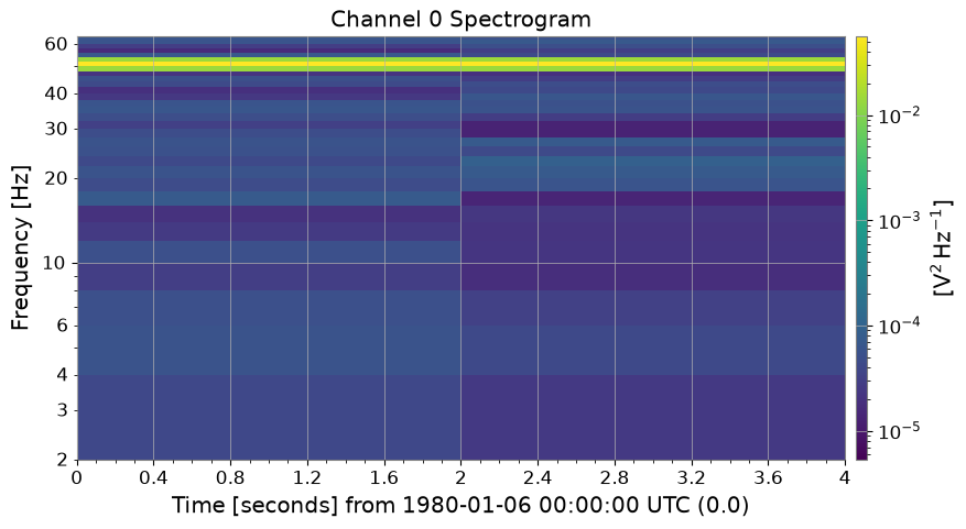
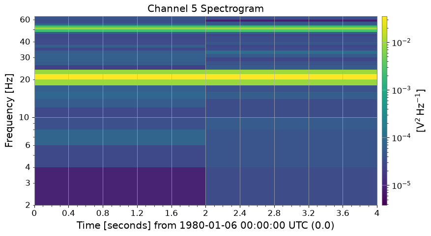
To plot only a specific channel, specify an index using the monitor argument.

# Plot the first channel (Channel_0)
plot0 = spec_matrix.plot(monitor=0, title="Channel 0 Spectrogram")
plot0.show()

# Plot the fifth channel (Channel_5)
plot5 = spec_matrix.plot(monitor=3, title="Channel 5 Spectrogram")
plot5.show()

5. Integration with External Libraries

For machine learning or GPU computing, the data can be easily converted to PyTorch or CuPy tensors.

# Conversion to PyTorch Tensor
try:
    import torch

    _ = torch
    torch_tensor = spec_matrix.to_torch()
    print("PyTorch Tensor:", type(torch_tensor))
    print("Shape:", torch_tensor.shape)
except ImportError:
    print("PyTorch is not installed.")

# Conversion to CuPy Array (if CUDA environment is available)
from gwexpy.interop import is_cupy_available

if is_cupy_available():
    cupy_array = spec_matrix.to_cupy()
    print("CuPy Array:", type(cupy_array))
    print("Shape:", cupy_array.shape)
else:
    pass

PyTorch is not installed.

Summary

• SpectrogramMatrix can be created using SpectrogramList.to_matrix().

• It holds data as a 3-dimensional array (Batch, Time, Freq).

• Methods like mean() and plot() make it easy to aggregate and visualize data.

• It serves as a useful intermediate format for passing data to deep learning frameworks via methods like to_torch().