Control Analysis: Discretization (ZOH vs Tustin)#
This notebook promotes the legacy control-theory example into the public docs set. The point is not just to call c2d(): it is to show how a continuous plant changes when a digital controller samples and holds actuator commands.
We compare Zero-Order Hold (ZOH) and Tustin because they preserve different physical aspects of the loop. ZOH is faithful to DAC-held commands in time-domain actuation, while Tustin tends to preserve frequency response near crossover more evenly.
import matplotlib.pyplot as plt
import numpy as np
from control.matlab import bode, c2d, step, tf

from gwexpy import FrequencySeries, TimeSeries

# Use a simple first-order plant so the discretization trade-off is easy to interpret physically.
P = tf([0, 1], [0.5, 1])
print(P)
<TransferFunction>: sys[0]
Inputs (1): ['u[0]']
Outputs (1): ['y[0]']

      1
  ---------
  0.5 s + 1
1. Discretize the plant#
Sampling does two things at once: it freezes actuator commands between updates and it warps the frequency axis seen by the digital filter. Those are different physical approximations, so we keep both versions.
ts = 0.2  # Sampling time [s]

# ZOH assumes the DAC holds each command constant until the next sample, which is often the right actuator model.
Pd_zoh = c2d(P, ts, method="zoh")

# Tustin maps the continuous pole/zero structure through a bilinear transform, which usually preserves loop-shape better near crossover.
Pd_tustin = c2d(P, ts, method="tustin")

print("ZOH:")
print(Pd_zoh)
print("Tustin:")
print(Pd_tustin)
ZOH:
<TransferFunction>: sys[0]$sampled
Inputs (1): ['u[0]']
Outputs (1): ['y[0]']
dt = 0.2

    0.3297
  ----------
  z - 0.6703
Tustin:
<TransferFunction>: sys[0]$sampled
Inputs (1): ['u[0]']
Outputs (1): ['y[0]']
dt = 0.2

  0.1667 z + 0.1667
  -----------------
     z - 0.6667
2. Compare frequency response#
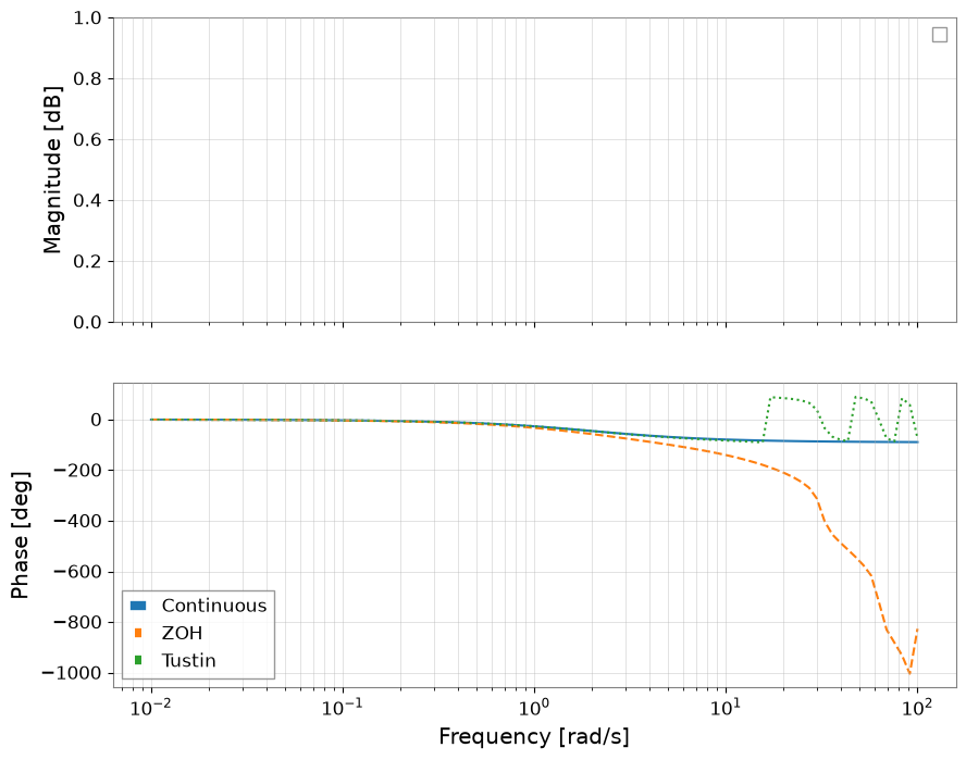
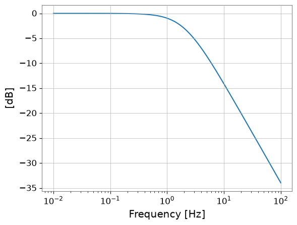
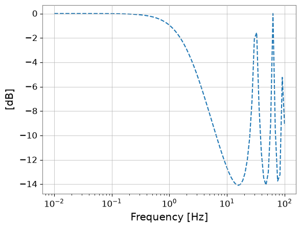
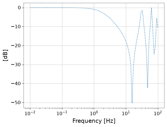
The physically important question is where phase and gain begin to drift away from the continuous plant. Excess phase error near the intended unity-gain region directly changes stability margin.
omega = np.logspace(-2, 2, 100)
mag_c, phase_c, w_c = bode(P, omega, plot=False)
mag_z, phase_z, w_z = bode(Pd_zoh, omega, plot=False)
mag_t, phase_t, w_t = bode(Pd_tustin, omega, plot=False)

fs_mag_c = FrequencySeries(20 * np.log10(mag_c), frequencies=w_c, unit="dB", name="Continuous")
fs_mag_z = FrequencySeries(20 * np.log10(mag_z), frequencies=w_z, unit="dB", name="ZOH")
fs_mag_t = FrequencySeries(20 * np.log10(mag_t), frequencies=w_t, unit="dB", name="Tustin")

fig, (ax1, ax2) = plt.subplots(2, 1, figsize=(10, 8), sharex=True)
fs_mag_c.plot(ax=ax1, label="Continuous")
fs_mag_z.plot(ax=ax1, label="ZOH", linestyle="--")
fs_mag_t.plot(ax=ax1, label="Tustin", linestyle=":")
ax1.set_xscale("log")
ax1.set_ylabel("Magnitude [dB]")
ax1.legend()
ax1.grid(which="both", alpha=0.5)

ax2.semilogx(w_c, np.rad2deg(phase_c), label="Continuous")
ax2.semilogx(w_z, np.rad2deg(phase_z), label="ZOH", linestyle="--")
ax2.semilogx(w_t, np.rad2deg(phase_t), label="Tustin", linestyle=":")
ax2.set_ylabel("Phase [deg]")
ax2.set_xlabel("Frequency [rad/s]")
ax2.legend()
ax2.grid(which="both", alpha=0.5)
plt.show()
/home/runner/micromamba/envs/gwexpy/lib/python3.11/site-packages/control/lti.py:138: UserWarning: __call__: evaluation above Nyquist frequency
  warn("__call__: evaluation above Nyquist frequency")
/home/runner/micromamba/envs/gwexpy/lib/python3.11/site-packages/control/lti.py:138: UserWarning: __call__: evaluation above Nyquist frequency
  warn("__call__: evaluation above Nyquist frequency")
3. Compare time response#
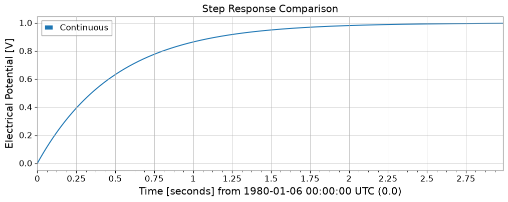
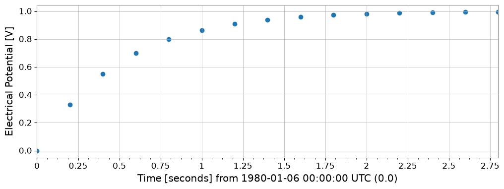
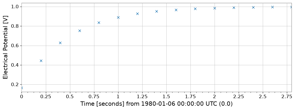
Time-domain comparisons reveal the other half of the story: ZOH reproduces held actuator commands naturally, while Tustin may look better in loop-shape analysis but can misrepresent the exact held-input waveform.
T_end = 3
Tc = np.arange(0, T_end, 0.01)
Td = np.arange(0, T_end, ts)

# Step response is a direct check of how the held-input assumption changes the plant's apparent settling behavior.
yc, tc = step(P, Tc)
yd_z, td_z = step(Pd_zoh, Td)
yd_t, td_t = step(Pd_tustin, Td)

ts_c = TimeSeries(yc, times=tc, unit="V", name="Continuous")
ts_z = TimeSeries(yd_z, times=td_z, unit="V", name="ZOH")
ts_t = TimeSeries(yd_t, times=td_t, unit="V", name="Tustin")

plot = ts_c.plot(label="Continuous", title="Step Response Comparison")
ax = plot.gca()
ts_z.plot(ax=ax, label="ZOH", marker="o", linestyle="None")
ts_t.plot(ax=ax, label="Tustin", marker="x", linestyle="None")
ax.legend()
ax.grid(True)
plt.show()