Control Analysis: Resonance and Feedback#
This notebook turns the legacy control measurement tutorial into a public control-analysis entrypoint. The core question is how to recognize a resonant plant from time-series data before any controller is designed.
We use a broadband drive, a second-order plant, ASD, coherence, and a measured transfer function. Those are the measurements that tell you whether the mode is real, where it sits, and whether the input truly explains the output.
import matplotlib.pyplot as plt
import numpy as np
import scipy.signal as signal

from gwexpy import TimeSeries

fs = 1024
duration = 60
t = np.arange(0, duration, 1 / fs)

# Broadband drive excites the plant across frequency, which is what makes system identification possible from one record.
np.random.seed(42)
u_data = np.random.randn(len(t))
u = TimeSeries(u_data, times=t, unit="V", name="Input (Drive)")

# A second-order resonance is a minimal model for a suspension or actuator mode: f0 sets the peak location and Q sets the ring-down width.
f0 = 10
Q = 10
w0 = 2 * np.pi * f0
num = [w0**2]
den = [1, w0 / Q, w0**2]
sys_dt = signal.cont2discrete((num, den), 1 / fs)
y_data = signal.dlti(sys_dt[0], sys_dt[1], dt=1 / fs).output(u.value, t=t)[1].flatten()
y = TimeSeries(y_data, times=t, unit="m", name="Output (Displacement)")
/home/runner/micromamba/envs/gwexpy/lib/python3.11/site-packages/scipy/signal/_ltisys.py:603: BadCoefficients: Badly conditioned filter coefficients (numerator): the results may be meaningless
  self.num, self.den = normalize(*system)
1. Inspect the time series#
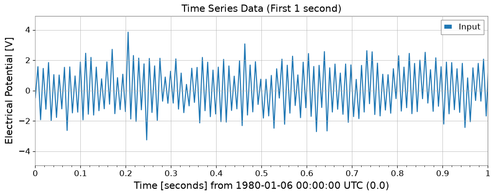
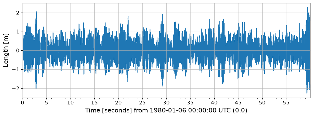
A short zoom shows that the output is not just delayed input: it rings because energy is temporarily stored in the resonant mode.
plot = u.plot(label="Input")
ax = plot.gca()
y.plot(ax=ax, label="Output")
ax.set_xlim(0, 1)
ax.legend()
ax.set_title("Time Series Data (First 1 second)")
plt.show()
2. ASD, coherence, and measured transfer function#
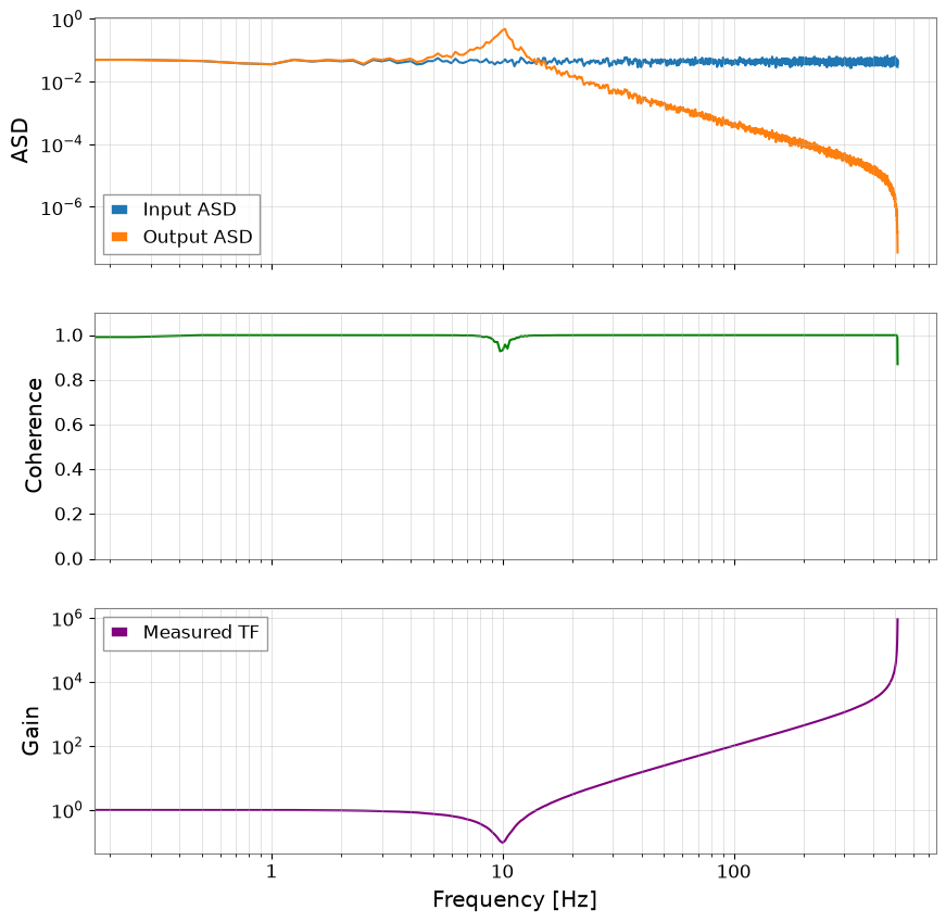
ASD shows where energy accumulates, coherence shows whether the drive really explains the response, and the transfer function combines both into the plant’s complex frequency response.
fftlength = 4

# Averaging 4-second chunks trades some frequency resolution for lower estimator variance.
asd_u = u.asd(fftlength=fftlength)
asd_y = y.asd(fftlength=fftlength)
coh = u.coherence(y, fftlength=fftlength)

# The transfer function is the quantity a controller designer actually wants: output motion per unit drive.
tf_meas = y.transfer_function(u, fftlength=fftlength)

fig, axes = plt.subplots(3, 1, figsize=(10, 10), sharex=True)
axes[0].loglog(asd_u, label="Input ASD")
axes[0].loglog(asd_y, label="Output ASD")
axes[0].legend()
axes[0].set_ylabel("ASD")
axes[0].grid(True, which="both", alpha=0.5)

axes[1].semilogx(coh.frequencies, coh.value, color="green")
axes[1].set_ylabel("Coherence")
axes[1].set_ylim(0, 1.1)
axes[1].grid(True, which="both", alpha=0.5)

axes[2].loglog(tf_meas.abs(), color="purple", label="Measured TF")
axes[2].set_ylabel("Gain")
axes[2].set_xlabel("Frequency [Hz]")
axes[2].legend()
axes[2].grid(True, which="both", alpha=0.5)
plt.show()