制御解析: 共振とフィードバック#
この notebook は legacy の計測・スペクトル解析チュートリアルを、公開 docs 用に共振解析の入口として整理したものです。コントローラを設計する前に知りたいのは、どこに共振があり、入力が本当に出力を説明しているか です。
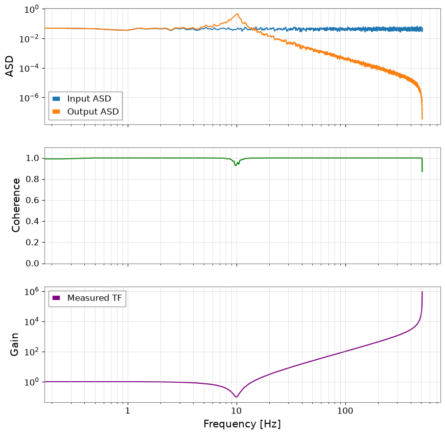
広帯域励振、2 次系のプラント、ASD、コヒーレンス、実測の伝達関数を用います。これらは、そのモードが実在するか、どの周波数にあるのか、入力が出力を本当に説明しているのかを教えてくれる測定量です。
import matplotlib.pyplot as plt
import numpy as np
import scipy.signal as signal

from gwexpy import TimeSeries

fs = 1024
duration = 60
t = np.arange(0, duration, 1 / fs)

# Broadband drive excites the plant across frequency, which is what makes system identification possible from one record.
np.random.seed(42)
u_data = np.random.randn(len(t))
u = TimeSeries(u_data, times=t, unit="V", name="Input (Drive)")

# A second-order resonance is a minimal model for a suspension or actuator mode: f0 sets the peak location and Q sets the ring-down width.
f0 = 10
Q = 10
w0 = 2 * np.pi * f0
num = [w0**2]
den = [1, w0 / Q, w0**2]
sys_dt = signal.cont2discrete((num, den), 1 / fs)
y_data = signal.dlti(sys_dt[0], sys_dt[1], dt=1 / fs).output(u.value, t=t)[1].flatten()
y = TimeSeries(y_data, times=t, unit="m", name="Output (Displacement)")
/home/runner/micromamba/envs/gwexpy/lib/python3.11/site-packages/scipy/signal/_ltisys.py:603: BadCoefficients: Badly conditioned filter coefficients (numerator): the results may be meaningless
  self.num, self.den = normalize(*system)
1. 時間波形を見る#
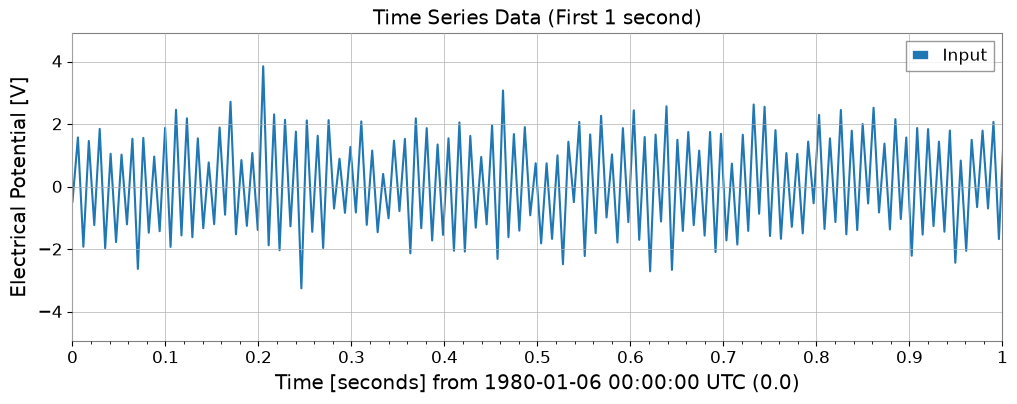
短時間のズームでは、出力が単なる遅れた入力ではなく、共振モードにエネルギーが一時的に蓄えられていることが見えます。
plot = u.plot(label="Input")
ax = plot.gca()
y.plot(ax=ax, label="Output")
ax.set_xlim(0, 1)
ax.legend()
ax.set_title("Time Series Data (First 1 second)")
plt.show()
2. ASD・コヒーレンス・伝達関数#
ASD はどこにエネルギーが集まるか、コヒーレンスは入力がどこまで出力を説明しているか、伝達関数はその両方をまとめた複素応答です。
fftlength = 4

# Averaging 4-second chunks trades some frequency resolution for lower estimator variance.
asd_u = u.asd(fftlength=fftlength)
asd_y = y.asd(fftlength=fftlength)
coh = u.coherence(y, fftlength=fftlength)

# The transfer function is the quantity a controller designer actually wants: output motion per unit drive.
tf_meas = y.transfer_function(u, fftlength=fftlength)

fig, axes = plt.subplots(3, 1, figsize=(10, 10), sharex=True)
axes[0].loglog(asd_u, label="Input ASD")
axes[0].loglog(asd_y, label="Output ASD")
axes[0].legend()
axes[0].set_ylabel("ASD")
axes[0].grid(True, which="both", alpha=0.5)

axes[1].semilogx(coh.frequencies, coh.value, color="green")
axes[1].set_ylabel("Coherence")
axes[1].set_ylim(0, 1.1)
axes[1].grid(True, which="both", alpha=0.5)

axes[2].loglog(tf_meas.abs(), color="purple", label="Measured TF")
axes[2].set_ylabel("Gain")
axes[2].set_xlabel("Frequency [Hz]")
axes[2].legend()
axes[2].grid(True, which="both", alpha=0.5)
plt.show()