制御解析: 離散化(ZOH と Tustin の比較)#
この notebook は legacy の制御理論例を公開 docs 用に整理したものです。ここで見たいのは c2d() の使い方そのものではなく、連続時間プラントがデジタル実装でどう見え方を変えるか です。
Zero-Order Hold (ZOH) は DAC が指令をサンプル間で保持するという物理モデルに対応し、Tustin は周波数応答の形を比較的よく保ちます。どちらを使うかで時間応答と位相余裕の見え方が変わります。
import matplotlib.pyplot as plt
import numpy as np
from control.matlab import bode, c2d, step, tf

from gwexpy import FrequencySeries, TimeSeries

# Use a simple first-order plant so the discretization trade-off is easy to interpret physically.
P = tf([0, 1], [0.5, 1])
print(P)
<TransferFunction>: sys[0]
Inputs (1): ['u[0]']
Outputs (1): ['y[0]']

      1
  ---------
  0.5 s + 1
1. プラントを離散化する#
サンプリングは「指令を保持する」という近似と、「周波数軸を写像する」という近似を同時に導入します。制御系ではこの 2 つを混同しないことが重要です。
ts = 0.2  # Sampling time [s]

# ZOH assumes the DAC holds each command constant until the next sample, which is often the right actuator model.
Pd_zoh = c2d(P, ts, method="zoh")

# Tustin maps the continuous pole/zero structure through a bilinear transform, which usually preserves loop-shape better near crossover.
Pd_tustin = c2d(P, ts, method="tustin")

print("ZOH:")
print(Pd_zoh)
print("Tustin:")
print(Pd_tustin)
ZOH:
<TransferFunction>: sys[0]$sampled
Inputs (1): ['u[0]']
Outputs (1): ['y[0]']
dt = 0.2

    0.3297
  ----------
  z - 0.6703
Tustin:
<TransferFunction>: sys[0]$sampled
Inputs (1): ['u[0]']
Outputs (1): ['y[0]']
dt = 0.2

  0.1667 z + 0.1667
  -----------------
     z - 0.6667
2. 周波数応答を比べる#
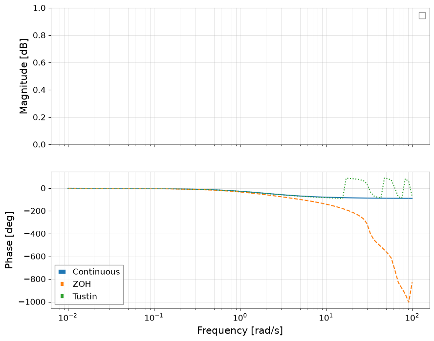
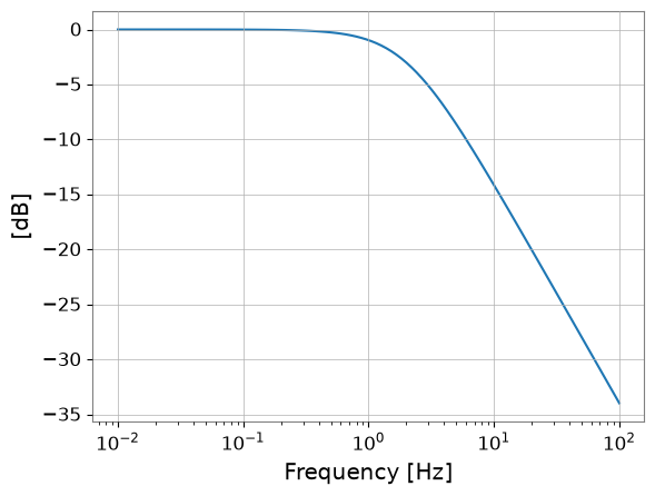
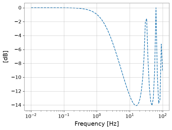
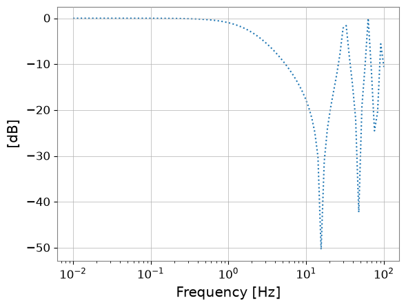
制御的に重要なのは、位相とゲインが連続系からどこでずれ始めるかです。とくに位相誤差は安定余裕を直接変えます。
omega = np.logspace(-2, 2, 100)
mag_c, phase_c, w_c = bode(P, omega, plot=False)
mag_z, phase_z, w_z = bode(Pd_zoh, omega, plot=False)
mag_t, phase_t, w_t = bode(Pd_tustin, omega, plot=False)

fs_mag_c = FrequencySeries(20 * np.log10(mag_c), frequencies=w_c, unit="dB", name="Continuous")
fs_mag_z = FrequencySeries(20 * np.log10(mag_z), frequencies=w_z, unit="dB", name="ZOH")
fs_mag_t = FrequencySeries(20 * np.log10(mag_t), frequencies=w_t, unit="dB", name="Tustin")

fig, (ax1, ax2) = plt.subplots(2, 1, figsize=(10, 8), sharex=True)
fs_mag_c.plot(ax=ax1, label="Continuous")
fs_mag_z.plot(ax=ax1, label="ZOH", linestyle="--")
fs_mag_t.plot(ax=ax1, label="Tustin", linestyle=":")
ax1.set_xscale("log")
ax1.set_ylabel("Magnitude [dB]")
ax1.legend()
ax1.grid(which="both", alpha=0.5)

ax2.semilogx(w_c, np.rad2deg(phase_c), label="Continuous")
ax2.semilogx(w_z, np.rad2deg(phase_z), label="ZOH", linestyle="--")
ax2.semilogx(w_t, np.rad2deg(phase_t), label="Tustin", linestyle=":")
ax2.set_ylabel("Phase [deg]")
ax2.set_xlabel("Frequency [rad/s]")
ax2.legend()
ax2.grid(which="both", alpha=0.5)
plt.show()
/home/runner/micromamba/envs/gwexpy/lib/python3.11/site-packages/control/lti.py:138: UserWarning: __call__: evaluation above Nyquist frequency
  warn("__call__: evaluation above Nyquist frequency")
/home/runner/micromamba/envs/gwexpy/lib/python3.11/site-packages/control/lti.py:138: UserWarning: __call__: evaluation above Nyquist frequency
  warn("__call__: evaluation above Nyquist frequency")
3. 時間応答を比べる#
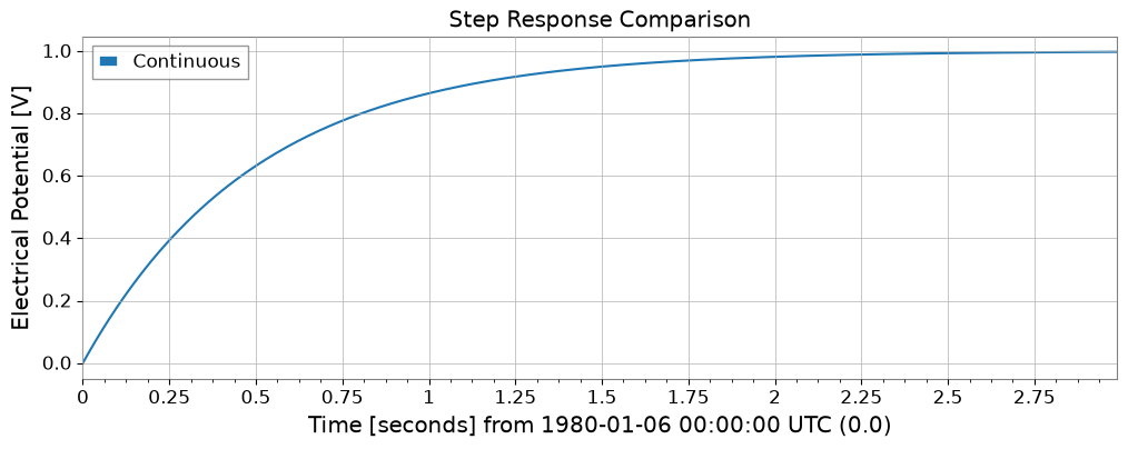
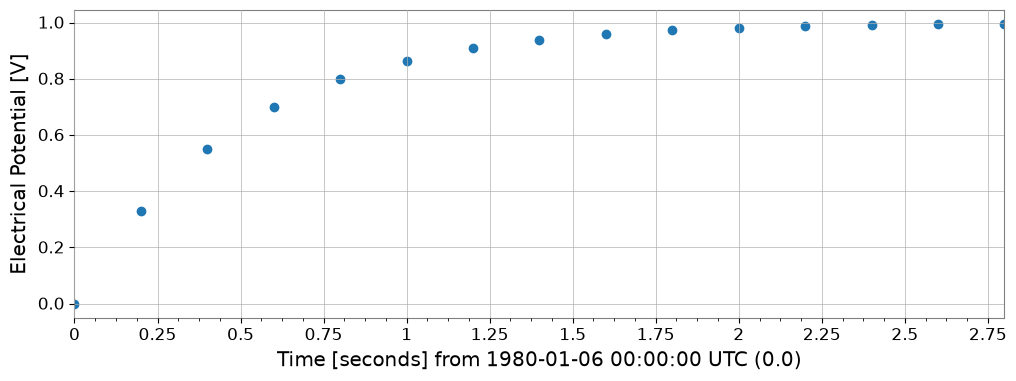
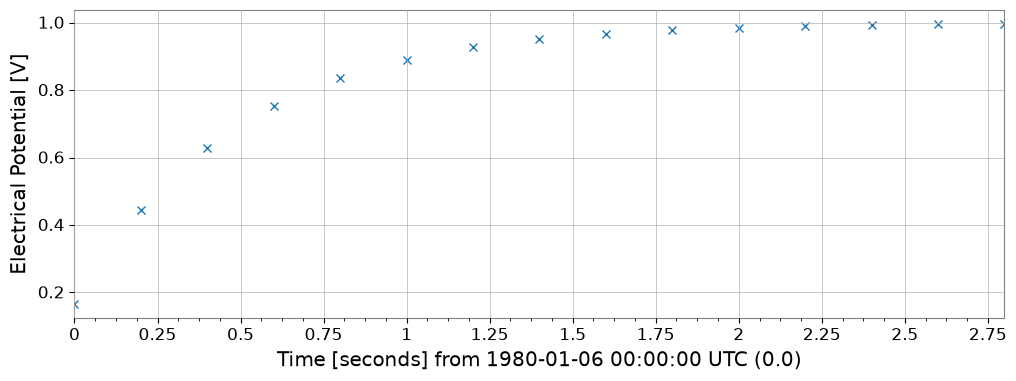
時間領域では ZOH が「保持された指令」を自然に再現し、Tustin は loop shape には有利でも保持入力の忠実度は別問題であることが見えてきます。
T_end = 3
Tc = np.arange(0, T_end, 0.01)
Td = np.arange(0, T_end, ts)

# Step response is a direct check of how the held-input assumption changes the plant's apparent settling behavior.
yc, tc = step(P, Tc)
yd_z, td_z = step(Pd_zoh, Td)
yd_t, td_t = step(Pd_tustin, Td)

ts_c = TimeSeries(yc, times=tc, unit="V", name="Continuous")
ts_z = TimeSeries(yd_z, times=td_z, unit="V", name="ZOH")
ts_t = TimeSeries(yd_t, times=td_t, unit="V", name="Tustin")

plot = ts_c.plot(label="Continuous", title="Step Response Comparison")
ax = plot.gca()
ts_z.plot(ax=ax, label="ZOH", marker="o", linestyle="None")
ts_t.plot(ax=ax, label="Tustin", marker="x", linestyle="None")
ax.legend()
ax.grid(True)
plt.show()