ケーススタディ: GBD 形式 I/O#
このチュートリアルでは、GBD ファイルの読み込みと書き出しについて解説します。GBD は、KAGRA 等の実験において PEM(環境モニタリング)に広く使用されている GRAPHTEC 製データロガー (GL シリーズ) のネイティブバイナリ形式です。
GBD とは?#
GBD (GRAPHTEC Binary Data) は以下のような特徴を持つ独自形式です:
メタデータを含む ASCII ヘッダー(チャンネル名、サンプリングレート、ローカル時刻、振幅レンジ等)
バイナリデータブロック(モデルにより float32 または int16)
マルチチャンネル記録(最大 32 チャンネル同時記録)
任意のデジタル(ロジック)チャンネル
レガシー移行に関する注記: レガシー KAGRA リポジトリにあった gbd2gwf.py および read_gbd.py スクリプトは gwexpy.timeseries.io.gbd に統合されました。 現在の公開ダイレクト I/O 契約については ファイル I/O 対応フォーマットガイド を参照してください。
import warnings


import tempfile
from pathlib import Path

import matplotlib.pyplot as plt
import numpy as np

from gwexpy.timeseries import TimeSeries, TimeSeriesDict, TimeSeriesMatrix
1. デモンストレーション用合成 GBD ファイルの作成#
実機がなくても実行できるように、最小限の有効な GBD ファイルを合成します。
GBD の構造は以下の通りです:
[ASCII Header]  (fixed HeaderSize bytes)
[Binary Data]   (N_counts × N_channels × itemsize bytes)
def make_synthetic_gbd(path: Path, n_samples: int = 10000, fs: float = 1000.0):
    """Write a minimal synthetic GBD file (GRAPHTEC GL-series format)."""
    rng = np.random.default_rng(7)
    t = np.arange(n_samples) / fs

    ch0 = 2.0 * np.sin(2 * np.pi * 10.0 * t) + 0.1 * rng.normal(0, 1, n_samples)   # 10 Hz
    ch1 = 1.5 * np.sin(2 * np.pi * 50.0 * t) + 0.1 * rng.normal(0, 1, n_samples)   # 50 Hz
    ch2 = np.where(np.sin(2 * np.pi * 1.0 * t) > 0, 1.0, 0.0).astype(np.float32)   # digital trigger

    local_start = "2023-05-20 14:30:00.000"
    local_stop  = f"2023-05-20 14:30:{n_samples / fs:.3f}"

    header_lines = [
        "[Header]",
        "HeaderSize = 1024",
        f"Start = {local_start}",
        f"Stop  = {local_stop}",
        f"Sample = {1000.0 / fs:.3f}ms",
        "Type = little,float32",
        "Order = CH0, CH1, CH2_LOGIC",
        f"Counts = {n_samples}",
        "$AMP",
        "CH0 = , , 10V",
        "CH1 = , , 5V",
        "CH2_LOGIC = , , 1V",
    ]
    header_str = "\r\n".join(header_lines) + "\r\n"
    header_bytes = header_str.encode("ascii")
    # Pad to 1024 bytes
    header_bytes = header_bytes.ljust(1024, b"\x00")

    # Data block: interleaved float32 (N_samples × N_channels)
    data = np.stack([ch0, ch1, ch2], axis=1).astype(np.float32)  # (N, 3)

    with open(path, "wb") as f:
        f.write(header_bytes)
        f.write(data.tobytes())

    print(f"Written: {path}  ({path.stat().st_size / 1024:.1f} KB)")


# Write to a temporary file
tmpdir = Path(tempfile.mkdtemp())
gbd_path = tmpdir / "synthetic_pem.gbd"
make_synthetic_gbd(gbd_path, n_samples=10000, fs=1000.0)
Written: /tmp/tmpdbdux8wj/synthetic_pem.gbd (118.2 KB)
2. TimeSeriesDict への読み込み#
TimeSeriesDict.read() で format='gbd' を指定します。GBD 内の時刻はローカルタイムで記録されているため、timezone パラメータが必要になります。
# Read all channels
tsd = TimeSeriesDict.read(
    str(gbd_path),
    format='gbd',
    timezone='Asia/Tokyo',   # JST (UTC+9) – required for GPS time conversion
)

print("Channels read:", list(tsd.keys()))
for name, ts in tsd.items():
    print(f"  {name:15s}: {len(ts.value):6d} samples, dt={ts.dt}, unit={ts.unit}")
Channels read: ['CH0', 'CH1', 'CH2_LOGIC']
  CH0            :  10000 samples, dt=0.001 s, unit=V
  CH1            :  10000 samples, dt=0.001 s, unit=V
  CH2_LOGIC      :  10000 samples, dt=0.001 s, unit=V
# Read only specific channels
tsd_subset = TimeSeriesDict.read(
    str(gbd_path),
    format='gbd',
    timezone='Asia/Tokyo',
    channels=['CH0', 'CH1'],   # only analog channels
)

print("Subset channels:", list(tsd_subset.keys()))
Subset channels: ['CH0', 'CH1']
# Read a single TimeSeries
ts_ch0 = TimeSeries.read(
    str(gbd_path),
    format='gbd',
    timezone='Asia/Tokyo',
    channels=['CH0'],
)

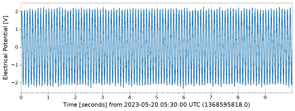
print(f"CH0: t0={ts_ch0.t0:.3f}, dt={ts_ch0.dt}, N={len(ts_ch0.value)}")

ts_ch0.plot(xscale='seconds');
CH0: t0=1368595818.000 s, dt=0.001 s, N=10000
3. GBD データに対する解析#
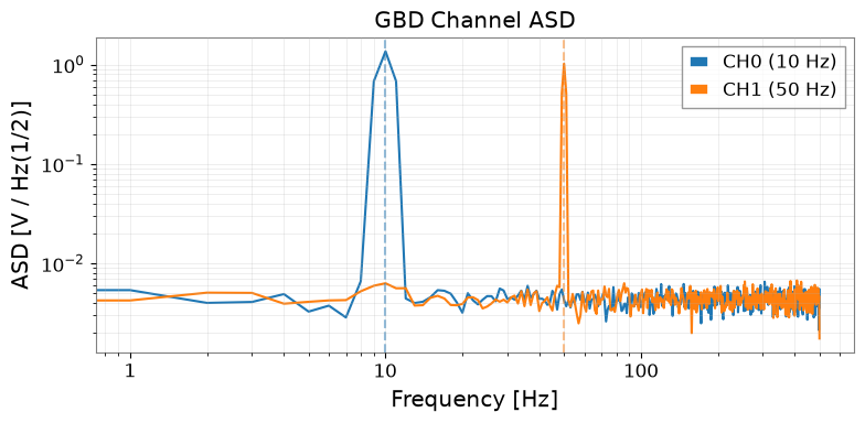
読み込まれたデータは標準的な gwexpy オブジェクトであるため、すべての解析メソッドが利用可能です。
ts_ch0 = tsd['CH0']
ts_ch1 = tsd['CH1']

# ASD comparison
asd_ch0 = ts_ch0.asd(fftlength=1.0, overlap=0.5)
asd_ch1 = ts_ch1.asd(fftlength=1.0, overlap=0.5)

fig, ax = plt.subplots(figsize=(8, 4))
ax.loglog(asd_ch0.frequencies.value, asd_ch0.value, label='CH0 (10 Hz)')
ax.loglog(asd_ch1.frequencies.value, asd_ch1.value, label='CH1 (50 Hz)')
ax.axvline(10,  color='C0', linestyle='--', alpha=0.5)
ax.axvline(50,  color='C1', linestyle='--', alpha=0.5)
ax.set_xlabel('Frequency [Hz]')
ax.set_ylabel(f'ASD [{asd_ch0.unit}]')
ax.set_title('GBD Channel ASD')
ax.legend()
ax.grid(True, which='both', alpha=0.3)
plt.tight_layout()
# Spectrogram of CH0
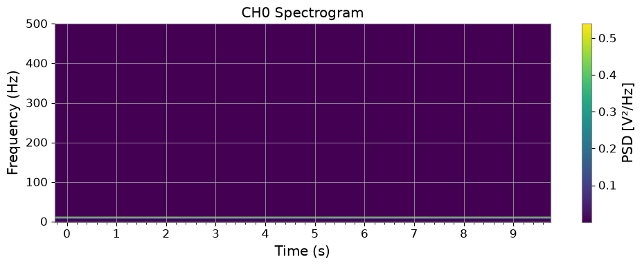
sg = ts_ch0.spectrogram(stride=0.5, fftlength=0.4, overlap=0.2)

fig, ax = plt.subplots(figsize=(10, 4))
mesh = ax.pcolormesh(
    sg.times.value,
    sg.frequencies.value,
    sg.value.T,
    shading='auto',
)
ax.set_xscale('auto-gps')
ax.set_xlabel('Time (s)')
ax.set_ylabel('Frequency (Hz)')
ax.set_title('CH0 Spectrogram')
plt.colorbar(mappable=mesh, ax=ax, label='PSD [V²/Hz]')
plt.tight_layout()
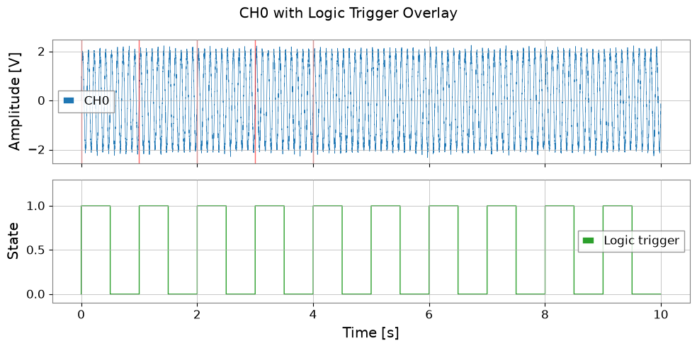
# Digital channel: use as event trigger
ts_logic = tsd['CH2_LOGIC']

# Find trigger-on times (0→1 transitions)
logic_val = ts_logic.value
transitions = np.where(np.diff(logic_val) > 0.5)[0]  # rising edges

t_axis = np.arange(len(logic_val)) * ts_logic.dt.value
trigger_times = t_axis[transitions]

print(f"Logic trigger ON events: {len(trigger_times)}")

fig, axes = plt.subplots(2, 1, figsize=(10, 5), sharex=True)
axes[0].plot(t_axis, ts_ch0.value, lw=0.5, label='CH0')
for tt in trigger_times[:5]:
    axes[0].axvline(tt, color='red', alpha=0.6, lw=1.0)
axes[0].set_ylabel('Amplitude [V]')
axes[0].legend()

axes[1].step(t_axis, logic_val, where='post', color='C2', lw=1.0, label='Logic trigger')
axes[1].set_xlabel('Time [s]')
axes[1].set_ylabel('State')
axes[1].set_ylim(-0.1, 1.3)
axes[1].legend()

plt.suptitle('CH0 with Logic Trigger Overlay')
plt.tight_layout()
Logic trigger ON events: 10
4. TimeSeriesMatrix による読み込み#
一括分析を行う場合は、TimeSeriesMatrix に直接読み込むことができます。
# Read all analog channels as TimeSeriesMatrix
tsm = TimeSeriesMatrix.read(
    str(gbd_path),
    format='gbd',
    timezone='Asia/Tokyo',
    channels=['CH0', 'CH1'],
)

print("TimeSeriesMatrix shape:", tsm.shape)  # (2, 1, N)

# ASD of all channels at once
try:
    asd_all = tsm.asd(fftlength=1.0, overlap=0.5)
    asd_all.plot(subplots=True)
except AttributeError:
    # GBD reader may create irregular time axis; fall back to per-channel ASD
    _asds = {name: tsd[name].asd(fftlength=1.0, overlap=0.5) for name in list(tsd.keys())[:2]}
    print("Per-channel ASD:", {k: f"{v.df.value:.4f} Hz/bin" for k, v in _asds.items()})
TimeSeriesMatrix shape: (2, 1, 10000)
Per-channel ASD: {'CH0': '1.0000 Hz/bin', 'CH1': '1.0000 Hz/bin'}
5. タイムゾーンの扱い#
GBD ファイルにはローカル時刻が格納されています。gwexpy は timezone パラメータを使用してこれらを自動的に GPS 時刻(UTC ベース)に変換します。
タイムゾーン |
IANA 名 |
UTC オフセット |
|---|---|---|
日本標準時 (KAGRA) |
|
+09:00 |
米国東部 (LIGO Hanford/LLO) |
|
−05:00 / −04:00 |
イタリア/欧州 (Virgo) |
|
+01:00 / +02:00 |
UTC |
|
±00:00 |
# Check GPS start time resulting from timezone conversion
tsd_jst = TimeSeriesDict.read(str(gbd_path), format='gbd', timezone='Asia/Tokyo')
tsd_utc = TimeSeriesDict.read(str(gbd_path), format='gbd', timezone='UTC')

t0_jst = tsd_jst['CH0'].t0
t0_utc = tsd_utc['CH0'].t0
print(f"t0 (JST→GPS): {t0_jst:.3f}")
print(f"t0 (UTC→GPS): {t0_utc:.3f}")
print(f"Difference: {(t0_jst - t0_utc).value:.1f} s  (should be 9×3600 = 32400 s)")
t0 (JST→GPS): 1368595818.000 s
t0 (UTC→GPS): 1368628218.000 s
Difference: -32400.0 s  (should be 9×3600 = 32400 s)
6. 移行ガイド: 従来の gbd2gwf.py → gwexpy#
Before (従来のスクリプト):
# gbd2gwf.py style
import numpy as np
from gwpy.timeseries import TimeSeries, TimeSeriesDict

# Manual header parsing
with open('data.gbd', 'rb') as f:
    header = f.read(1024).decode('ascii')
    # ... parse Start, Sample, Order, Counts by hand ...
    n_ch = len(channels)
    data = np.frombuffer(f.read(), dtype='<f4').reshape(-1, n_ch)

# Manual GPS time conversion
import pytz
from gwpy.time import to_gps
tz = pytz.timezone('Asia/Tokyo')
t_local = datetime.strptime(start_str, '%Y-%m-%d %H:%M:%S')
t_utc = tz.localize(t_local).astimezone(pytz.utc)
gps_start = to_gps(t_utc.strftime('%Y-%m-%dT%H:%M:%S'))

# Build dict manually
tsd = TimeSeriesDict()
for i, ch in enumerate(channels):
    tsd[ch] = TimeSeries(data[:, i] * scale[i], t0=gps_start, dt=dt)
移行後(gwexpy):
from gwexpy.timeseries import TimeSeriesDict

tsd = TimeSeriesDict.read(
    'data.gbd',
    format='gbd',
    timezone='Asia/Tokyo',
)
まとめ#
タスク |
API |
|---|---|
全チャンネル読み込み |
|
一部のみ読み込み |
|
単一チャンネル読み込み |
|
Matrix として読み出し |
|
デジタルチャンネルの自動検出 |
|
デジタルチャンネルの上書き指定 |
|
GPS エポックの上書き指定 |
|
関連チュートリアル: