開発版ドキュメント · 0.2.3 30c2f8ba · 入門例の検証対象 0.2.3 · 版情報 · 既知の制限

Bruco: コヒーレンス解析

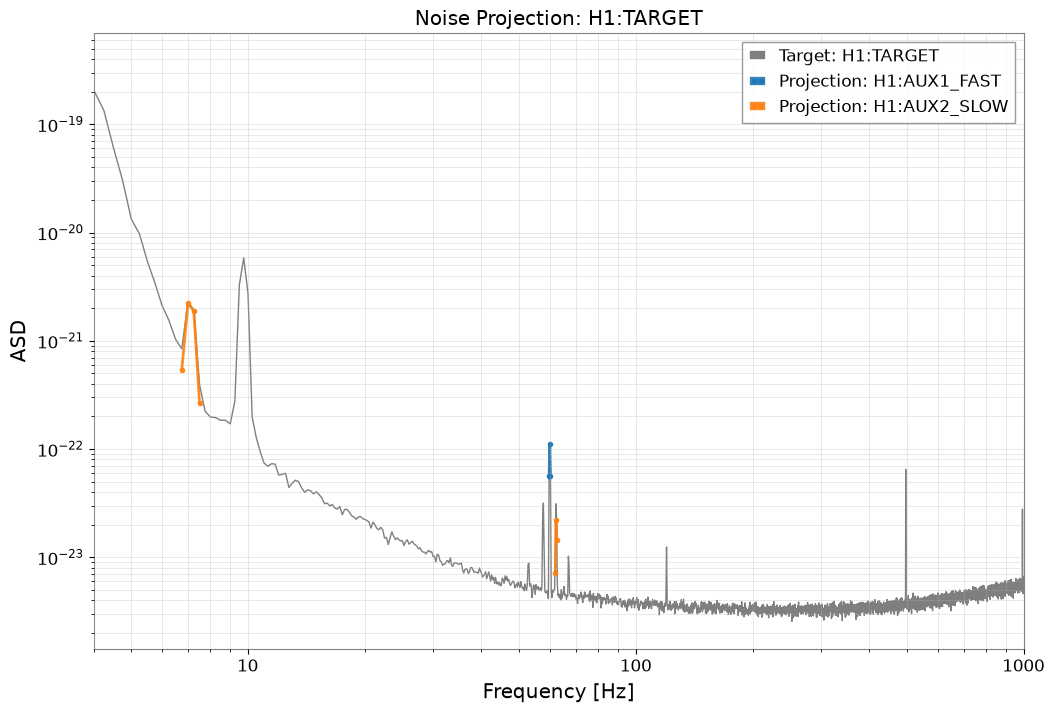
Brucoは**「総当たりコヒーレンス（Brute force coherence）」**を計算するためのツールです。重力波検出器（LIGOやVirgo）の主チャンネル（ターゲット）と、多数の補助チャンネルとの間のコヒーレンスを計算し、ノイズ源を特定することを目的としています。 物理的な狙いは、単に相関ランキングを作ることではなく、特定の周波数帯の DARM 過剰パワーを説明できる補助チャンネル候補を見つけ、実際に対処可能な結合経路へ結び付けることです。

並列処理によるコヒーレンス計算

Pythonの multiprocessing モジュールを使用して複数のCPUコアで並列実行されます。

1. タスク分割: 全補助チャンネルリストをCPU数に応じて分割し、各プロセスに割り当てます。

2. データ取得と前処理:

   • 各補助チャンネルのデータを取得します。

   • データが一定（フラット）の場合はスキップします。

   • サンプリングレートが出力要求レート (outfs) より高い場合、decimate 関数を用いてダウンサンプリングします。

3. コヒーレンス算出:

   • 補助チャンネルのFFTとPSD（パワースペクトル密度）を計算します。

   • ターゲットチャンネルとのCSD（クロススペクトル密度）を計算します。

   • コヒーレンス を以下の式で計算します：

4. Top N の選出:

   • すべての周波数ビンについて、計算されたコヒーレンス値が既存の上位リスト（top）よりも高い場合、その値を更新します。これにより、全チャンネルの結果を保持するのではなく、相関の高い上位チャンネルのみを効率的に記録します。

5. 結果の集約と出力:

   • 各プロセスから返された cohtab（コヒーレンス値）と idxtab（チャンネルID）を結合・ソートし、最終的な上位リストを作成します。

   • HTMLレポート作成: markup.py を使用して index.html を生成します。これには、周波数ごとの上位相関チャンネルの表（ヒートマップ形式の着色あり）や、プロット画像へのリンクが含まれます。

   • プロット作成: matplotlib を使用して、コヒーレンスとスペクトルのグラフ（PNGまたはPDF）を生成します。

この実装は、大量のチャンネルデータを効率的に処理するために、FFTの事前計算、並列処理、およびメモリ効率の良いTop-N記録方式を採用している点が特徴です。

オリジナルのBruco実装は以下で公開されています。設計詳細やCLIの挙動を確認したい場合はこちらを参照してください。

• https://github.com/mikelovskij/bruco

設計の詳細や CLI の挙動はこちらを参照してください。

このノートブックでは、対話的な解析・柔軟なデータ操作・高度な仮説検証を示すことで、gwexpy の Bruco モジュールを Python ライブラリとして 使う利点を紹介します。

• 実データは使わず、gwpy / numpy で生成した擬似データを利用します。

• CLI では難しい「非線形カップリング」や「変調」のシナリオに対する迅速な仮説検証を、Python API を用いて示します。

よくある誤り: 大きなコヒーレンスピークを因果的カップリングの証拠と解釈すること。コヒーレンスはランキングのための道具であり、証明ではありません。あるチャンネルに基づいて対処する前に、そのウィットネスが物理的に DARM の上流にあることを確認し、共通の駆動源がないか調べ、窓関数・前処理・セグメント選択を妥当な範囲で変えても特徴が残ることを確かめてください。

セットアップとモックデータ生成

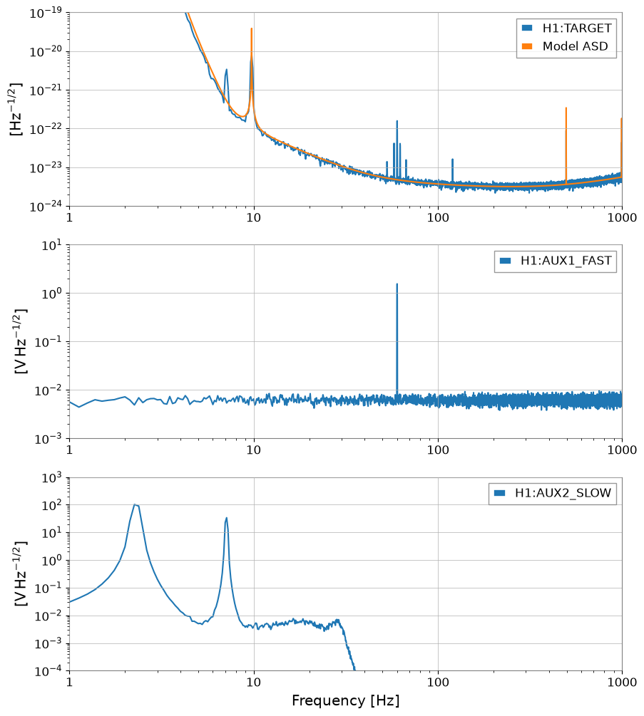
何をするか: ターゲット/補助チャンネルの擬似データを作り、Brucoに食わせるための TimeSeries を準備します。 なぜ重要か: 実運用ではNDSやフレームから取得しますが、ノートブック上で自由に信号を設計できると仮説検証が加速します。

import warnings

# ruff: noqa: I001
from astropy import units as u
import matplotlib.pyplot as plt
import numpy as np

from gwexpy.analysis import Bruco
from gwexpy.analysis.bruco import FastCoherenceEngine
from gwexpy.astro import inspiral_range
from gwexpy.frequencyseries import FrequencySeriesDict
from gwexpy.noise.asd import from_pygwinc
from gwexpy.noise.wave import from_asd
from gwexpy.plot import Plot
from gwexpy.timeseries import TimeSeries, TimeSeriesDict

rng = np.random.default_rng(7)

duration = 128  # seconds
sample_rate = 2048  # Hz
fftlength = 4.0  # seconds
overlap = 2.0  # seconds

t = np.arange(0, duration, 1 / sample_rate)

# Get aLIGO sensitivity curve (ASD)
fmax = sample_rate / 2  # Nyquist frequency
asd_aligo = from_pygwinc(
    "aLIGO", fmin=4.0, fmax=fmax, df=1.0 / duration, quantity="strain"
)

# Generate target noise based on aLIGO sensitivity curve
target = from_asd(asd_aligo, duration, sample_rate, t0=0, rng=rng).highpass(1)
target.channel = "H1:TARGET"

# Signals for auxiliary channels
fast_line = np.sin(2 * np.pi * 60.0 * t)
slow_motion = 70 * np.sin(2 * np.pi * 2.3 * t) + 30 * np.sin(2 * np.pi * 7.1 * t)

aux1_data = 0.8 * fast_line + 0.2 * rng.normal(0, 1.0, size=t.size)
aux2_data = 0.9 * slow_motion + 0.2 * rng.normal(0, 1.0, size=t.size) + 1
aux1 = TimeSeries(
    aux1_data, sample_rate=sample_rate, t0=0, unit="V", channel="H1:AUX1_FAST"
)
aux2 = TimeSeries(
    aux2_data, sample_rate=sample_rate, t0=0, unit="V", channel="H1:AUX2_SLOW"
).lowpass(30)

# Injection signal into target: aLIGO-based noise + linear coupling + nonlinear injection
target = target + 1e-22 * target.unit * (
    aux1 / u.V + aux2 / u.V + (aux1 / u.V / 2) ** 2 + 0.01 * (aux1 * aux2 / u.V**2)
)


target.name = target.channel
aux1.name = aux1.channel
aux2.name = aux2.channel

aux_dict = TimeSeriesDict(
    {
        aux1.channel: aux1,
        aux2.channel: aux2,
    }
)

print(f"aLIGO ASD at 100 Hz: {asd_aligo.crop(99, 101).value[0]:.2e} strain/sqrt(Hz)")
print(f"Target data std: {target.std():.2e}")

plot = Plot(
    [target.asd(8, 4), asd_aligo],
    aux1.asd(8, 4),
    aux2.asd(8, 4),
    figsize=(10, 12),
    sharex=True,
)
axes = plot.get_axes()
axes[0].set_xlim(1, 1e3)
axes[0].set_ylim(1e-24, 1e-19)
axes[1].set_ylim(1e-3, 1e1)
axes[2].set_ylim(1e-4, 1e3)
axes[0].legend([target.name, "Model ASD"])
axes[1].legend([aux1.name])
axes[2].legend([aux2.name])

aLIGO ASD at 100 Hz: 3.71e-24 strain/sqrt(Hz)
Target data std: 5.08e-19

<matplotlib.legend.Legend at 0x7fe22da69d10>

Section 1: 基本的なBruco解析の実行 (Jupyter上での再現)

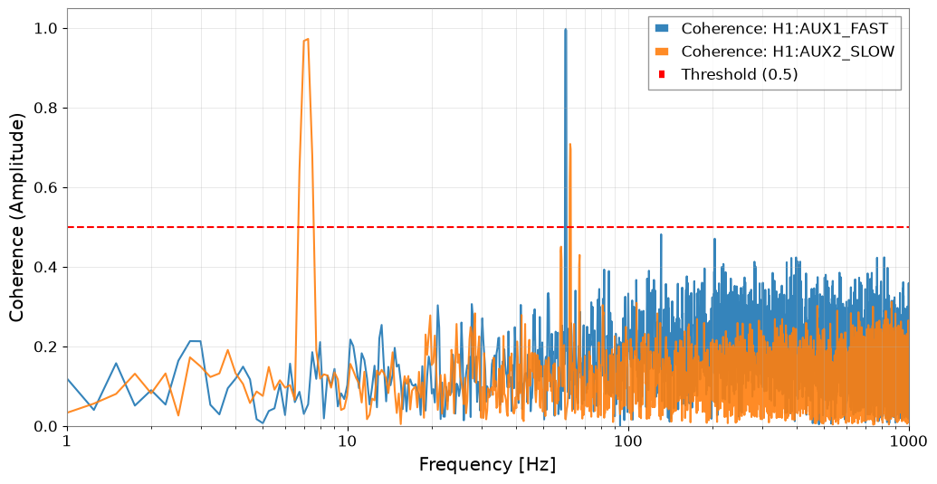
何をするか: Bruco クラスで総当たりコヒーレンス解析を実行し、結果をテーブルとプロットで確認します。 なぜ重要か: Python APIなら、対話的に条件や可視化を変えながら“犯人探し”を素早く試せます。

# Initialize Bruco.
# Since we manually pass all data here, specify an empty list for auto-fetch channel list (aux_channels).
bruco = Bruco(target_channel=target.name, aux_channels=[])

# By passing target_data and aux_data to the compute method, you can skip internal fetching and run the analysis.
result = bruco.compute(
    start=0,
    duration=int(duration),
    fftlength=fftlength,
    overlap=overlap,
    parallel=1,
    batch_size=2,
    top_n=3,
    target_data=target,  # Pre-generated target data
    aux_data=aux_dict,  # Pre-generated auxiliary channel data dictionary
)

df = result.to_dataframe(ranks=[0])

df_sorted = (
    df.sort_values("coherence", ascending=False)
    .dropna(subset=["channel"])
    .head(15)
    .reset_index(drop=True)
)

df_sorted

	frequency	rank	channel	coherence	projection
0	60.00	1	H1:AUX1_FAST	0.998699	1.118712e-22
1	59.75	1	H1:AUX1_FAST	0.994909	5.587699e-23
2	60.25	1	H1:AUX1_FAST	0.994519	5.570859e-23
3	7.25	1	H1:AUX2_SLOW	0.973445	1.888851e-21
4	7.00	1	H1:AUX2_SLOW	0.968398	2.211076e-21
5	62.25	1	H1:AUX2_SLOW	0.709532	2.210663e-23
6	62.50	1	H1:AUX2_SLOW	0.695847	1.435894e-23
7	7.50	1	H1:AUX2_SLOW	0.680465	2.682833e-22
8	6.75	1	H1:AUX2_SLOW	0.641778	5.413037e-22
9	62.00	1	H1:AUX2_SLOW	0.615101	7.153501e-24
10	131.25	1	H1:AUX1_FAST	0.482609	1.772034e-24
11	203.75	1	H1:AUX1_FAST	0.471606	1.572731e-24
12	57.75	1	H1:AUX2_SLOW	0.451528	1.428494e-23
13	57.50	1	H1:AUX2_SLOW	0.440484	9.442593e-24
14	67.25	1	H1:AUX2_SLOW	0.430697	3.624043e-24

result.plot_projection(coherence_threshold=0.5)
plt.xlim(4, 1000)
plt.show()

result.plot_coherence(coherence_threshold=0.5)
plt.xlim(1, 1000)
plt.show()

report_path = result.generate_report("bruco_report", coherence_threshold=0.4)
report_path

'bruco_report/index.html'

Section 2: 高度な前処理と仮説検証 (Deep Dive: Nonlinear & Bilinear)

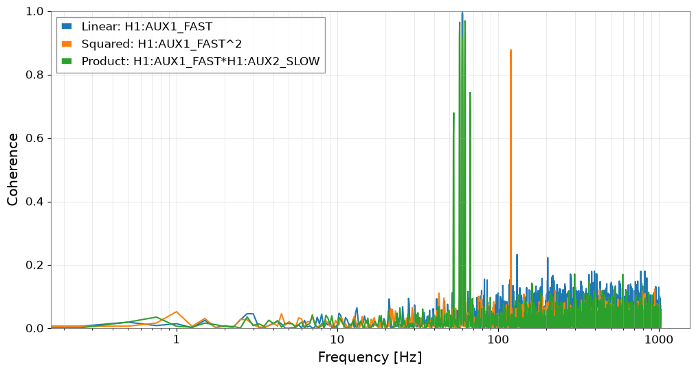
何をするか: 既存の線形相関だけでは説明できないノイズを想定し、非線形結合（2乗）や変調（積）を仮説として検定します。 なぜ重要か: FastCoherenceEngine を使うと、ターゲットのFFTを再計算せずに仮想チャンネルを高速に試せます。

物理的意図: こうした仮想チャンネルは fast × slow のような結合モデルを表し、高周波キャリアが低周波のアライメント変動・制御揺らぎ・環境ドリフトで変調される状況を検証します。

失敗しやすいパターン: ハイパス／バンドパスによる分離を省いて広帯域チャンネルを直接掛け合わせると、その積はしばしば無関係な低周波パワーに支配され、得られるコヒーレンスの解釈が難しくなります。

仮想ウィットネスを信頼する前のチェックリスト:

• ウィットネスの構成が妥当なカップリング機構に対応していること、

• 変調帯域が物理的に意味を持つ程度に十分狭いこと、

• 回復したコヒーレンスが、至る所ではなく、実際にサイドバンドやラインの揺らぎが存在する場所に現れること。

ts_sq = aux1**2
ts_sq.name = f"{aux1.name}^2"

ts_prod = aux1 * aux2
ts_prod.name = f"{aux1.name}*{aux2.name}"

engine = FastCoherenceEngine(target, fftlength=fftlength, overlap=overlap)

coh_linear = engine.compute_coherence(aux1)
coh_sq = engine.compute_coherence(ts_sq)
coh_prod = engine.compute_coherence(ts_prod)

freqs = engine.frequencies

fig, ax = plt.subplots(figsize=(12, 6))
ax.semilogx(freqs, coh_linear, label=f"Linear: {aux1.name}")
ax.semilogx(freqs, coh_sq, label=f"Squared: {ts_sq.name}")
ax.semilogx(freqs, coh_prod, label=f"Product: {ts_prod.name}")

ax.set_xlabel("Frequency [Hz]")
ax.set_ylabel("Coherence")
ax.set_ylim(0.0, 1.0)
ax.grid(True, which="both", ls="-", alpha=0.4)
ax.legend()
plt.show()

Section 3: 下流解析への接続 (Actionable Outcome)

何をするか: もっとも寄与が大きいノイズ仮説を用いて残差スペクトルを推定し、BNS Rangeの改善量を見積もります。 なぜ重要か: Bruco結果を“見つけて終わり”にせず、感度改善やノイズ除去ワークフローにつなげられます。

よくある誤り: 射影された残差を、保証された差し引き結果として読むこと。射影はウィットネスが代表性を持ち良条件であることを前提とします。ウィットネスが汚染されている、遅延がある、または断続的にしか結合していない場合、予測される改善は楽観的すぎることがあります。この節は、完全な差し引き検討の前のスクリーニングステップとして扱ってください。

target_asd = target.asd(fftlength=fftlength, overlap=overlap)
target_asd_vals = target_asd.value

coh_map = {
    aux1.name: coh_linear,
    ts_sq.name: coh_sq,
    ts_prod.name: coh_prod,
}

dominant_label = max(coh_map, key=lambda k: np.nanmax(coh_map[k]))
dominant_coh = coh_map[dominant_label]

# Estimate virtual channel contribution in ASD using Bruco's projection formula
projected_asd = target_asd_vals * np.sqrt(dominant_coh)
residual_asd_vals = np.sqrt(np.maximum(target_asd_vals**2 - projected_asd**2, 0.0))

residual_asd = target_asd.copy()
residual_asd.value[:] = residual_asd_vals

fig, ax = plt.subplots(figsize=(12, 6))
# ax.loglog(target_asd.frequencies.value, target_asd_vals, label="Target ASD")
# ax.loglog(target_asd.frequencies.value, residual_asd_vals, label="Residual ASD")
ax.loglog(target_asd, label="Target ASD")
ax.loglog(residual_asd, label="Residual ASD")
ax.set_xlabel("Frequency [Hz]")
ax.set_ylabel("ASD")
ax.grid(True, which="both", ls="-", alpha=0.4)
ax.legend()
plt.show()

# BNS Range comparison
bns_range_before = inspiral_range(target_asd**2, mass1=1.4, mass2=1.4, fmin=10)
bns_range_after = inspiral_range(residual_asd**2, mass1=1.4, mass2=1.4, fmin=10)

print(f"Dominant hypothesis: {dominant_label}")
print(f"BNS range (before): {bns_range_before.to_value(u.Mpc):.2f} Mpc")
print(f"BNS range (after):  {bns_range_after.to_value(u.Mpc):.2f} Mpc")

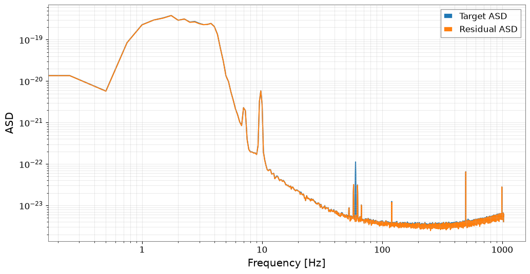
Dominant hypothesis: H1:AUX1_FAST
BNS range (before): 182.48 Mpc
BNS range (after):  186.24 Mpc

virtual_channels = {
    aux1.name: aux1,
    ts_sq.name: ts_sq,
    ts_prod.name: ts_prod,
}

culprit_channels = [dominant_label]
witnesses = TimeSeriesDict({name: virtual_channels[name] for name in culprit_channels})

spectral_options = dict(fftlength=8.0, overlap=4.0, window="hann", average="mean")
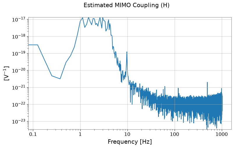
cxx = witnesses.csd_matrix(**spectral_options)
cyx = TimeSeriesDict({"TARGET": target}).csd_matrix(other=witnesses, **spectral_options)

# Cij = <conj(X_i) X_j>, so conjugate to map witnesses to TARGET.
# Use the same mean averaging for diagonal PSD and off-diagonal CSD entries.
H_lowres = (cyx @ cxx.inv()).conj()
for j, name in enumerate(culprit_channels):
    H_lowres.meta[0, j].unit = target.unit / witnesses[name].unit
    assert np.all(np.isfinite(H_lowres[0, j].value))

# Display estimated transfer function
H_lowres.abs().plot(xscale="log", yscale="log").suptitle("Estimated MIMO Coupling (H)")
plt.show()

# Full-resolution FFT


tsd = TimeSeriesDict({"MAIN": target, **witnesses})
aux_names = culprit_channels

tsd_fft = tsd.fft()
main_fft = tsd_fft["MAIN"]

# Filter interpolation and matrix operation
H = H_lowres.interpolate(main_fft.frequencies)
X_mat = FrequencySeriesDict({k: tsd_fft[k] for k in aux_names}).to_matrix()

# Projection and subtraction
Y_proj = (H @ X_mat)[0, 0]
assert Y_proj.unit == main_fft.unit
cleaned_fft = main_fft - Y_proj

# To time domain
cleaned_ts = cleaned_fft.ifft()

# Verify noise subtraction effect
fig = plt.figure(figsize=(12, 6))
ax = fig.gca()

# Overlay original and cleaned data (first 1 second)
plot_duration = 1.0
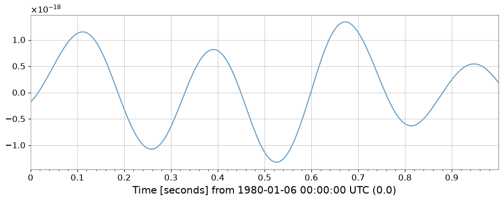
target.crop(end=target.t0.value + plot_duration).plot(
    ax=ax, label="Original", alpha=0.7
)  # noqa: F821
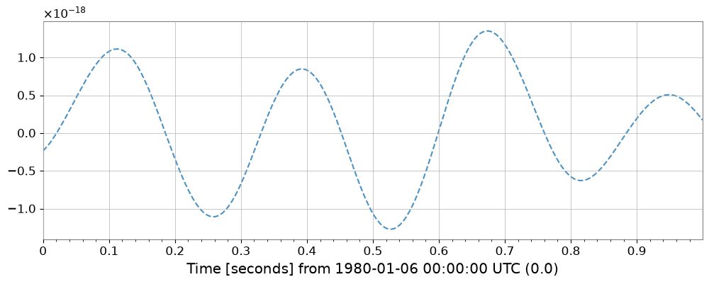
cleaned_ts.crop(end=target.t0.value + plot_duration).plot(
    ax=ax, label="Cleaned (Bruco)", linestyle="--", alpha=0.8
)  # noqa: F821

ax.set_title(f"Noise Subtraction Result (First {plot_duration}s)")
ax.legend(["Original", "Cleaned (Bruco)"])
plt.show()