信号抽出: 色付き雑音からの微弱信号回収#
このケーススタディは legacy の weak-signal notebook を公開 gallery 向けに整理したものです。物理的に見たいのは、生波形では見えない狭帯域信号をどうやって回収するかです。
ここでは弱い単色線を注入し、ASD で候補周波数を見つけ、band-pass で取り出してから簡単な正弦波モデルを当てます。
関連 API: Time Series API, Signal API
関連理論: 検証済みアルゴリズム、数値的安定性
import matplotlib.pyplot as plt
import numpy as np
np.random.seed(42)

from gwexpy import TimeSeries

duration = 32
sample_rate = 4096
signal_freq = 123.4
signal_amp = 0.5
noise_std = 5.0
t = np.linspace(0, duration, int(duration * sample_rate), endpoint=False)

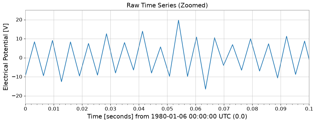
# The injected tone is far below the broadband noise floor, which is why it disappears in the raw waveform.
noise = np.random.normal(0, noise_std, size=len(t))
clean_signal = signal_amp * np.sin(2 * np.pi * signal_freq * t)
ts = TimeSeries(noise + clean_signal, t0=0, sample_rate=sample_rate, name="Noisy Data", unit="V")
1. 候補帯域を見つける#
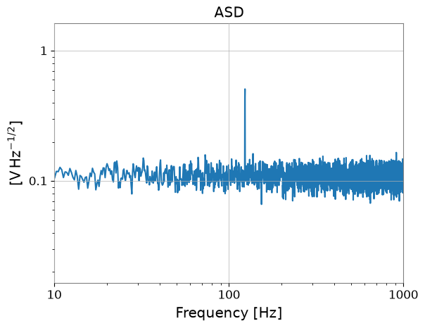
ASD の平均化は推定分散を減らすので、時間波形では見えない狭帯域線が統計的に見えるようになります。
plot = ts.plot()
plot.gca().set_xlim(0, 0.1)
plot.gca().set_title("Raw Time Series (Zoomed)")
plt.show()

asd = ts.asd(fftlength=4, method="welch")
plot = asd.plot()
plot.gca().set_xlim(10, 1000)
plot.gca().set_yscale("log")
plot.gca().set_title("ASD")
plt.show()
2. フィルタしてフィットする#
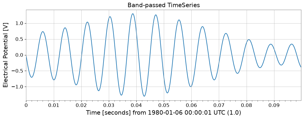
band-pass は注入線を残しつつ不要な広帯域成分を落とすためのものです。帯域を狭くしすぎると波形を歪め、広くしすぎると雑音を戻してしまいます。
関連 API: Time Series API, Fitting API
関連理論: 検証済みアルゴリズム
# Keep the band around the detected line so the fit sees the signal-dominated portion of the data.
filtered_ts = ts.bandpass(110, 130).crop(1, 1.1)

plot = filtered_ts.plot()
plot.gca().set_title("Band-passed TimeSeries")
plt.show()

def sine_model(t, amp, freq, phase, amp2, freq2, phase2):
    return amp * np.sin(2 * np.pi * freq * t + phase) * (1 + amp2 * np.sin(2 * np.pi * freq2 * t + phase2))

p0 = {"amp": 0.5, "freq": 123, "phase": 0, "amp2": 0.05, "freq2": 10, "phase2": 0}
limits = {"freq": (110, 130), "amp": (0.1, 5), "amp2": (0, 0.2), "freq2": (0, 50)}
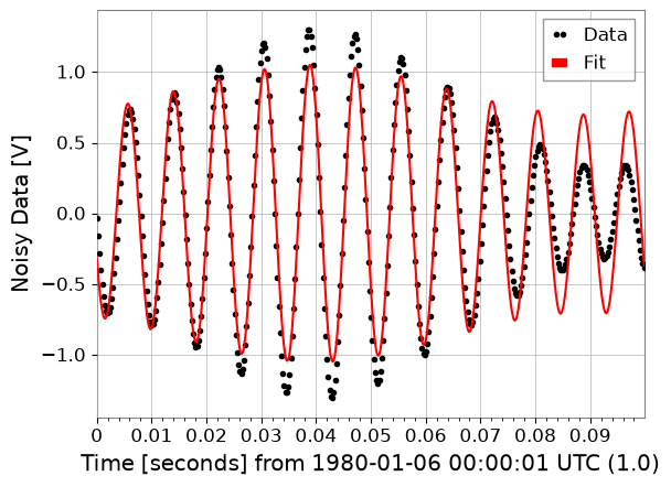
result = filtered_ts.fit(sine_model, p0=p0, limits=limits, sigma=0.01)
print(result)
result.plot()
plt.show()
┌─────────────────────────────────────────────────────────────────────────┐
│                                Migrad                                   │
├──────────────────────────────────┬──────────────────────────────────────┤
│ FCN = 1.414e+05 (χ²/ndof = 350.1)│              Nfcn = 456              │
│ EDM = 1.72e-05 (Goal: 0.0002)    │                                      │
├──────────────────────────────────┼──────────────────────────────────────┤
│          Valid Minimum           │   Below EDM threshold (goal x 10)    │
├──────────────────────────────────┼──────────────────────────────────────┤
│     SOME parameters at limit     │           Below call limit           │
├──────────────────────────────────┼──────────────────────────────────────┤
│             Hesse ok             │         Covariance accurate          │
└──────────────────────────────────┴──────────────────────────────────────┘
┌───┬────────┬───────────┬───────────┬────────────┬────────────┬─────────┬─────────┬───────┐
│   │ Name   │   Value   │ Hesse Err │ Minos Err- │ Minos Err+ │ Limit-  │ Limit+  │ Fixed │
├───┼────────┼───────────┼───────────┼────────────┼────────────┼─────────┼─────────┼───────┤
│ 0 │ amp    │ 875.0e-3  │  0.7e-3   │            │            │   0.1   │    5    │       │
│ 1 │ freq   │  120.314  │   0.006   │            │            │   110   │   130   │       │
│ 2 │ phase  │   20.46   │   0.04    │            │            │         │         │       │
│ 3 │ amp2   │200.000e-3 │ 0.002e-3  │            │            │    0    │   0.2   │       │
│ 4 │ freq2  │  10.101   │   0.020   │            │            │    0    │   50    │       │
│ 5 │ phase2 │   -1.59   │   0.13    │            │            │         │         │       │
└───┴────────┴───────────┴───────────┴────────────┴────────────┴─────────┴─────────┴───────┘
┌────────┬─────────────────────────────────────────────────────────────┐
│        │       amp      freq     phase      amp2     freq2    phase2 │
├────────┼─────────────────────────────────────────────────────────────┤
│    amp │  5.56e-07         0   -0.3e-6 -0.03e-15    5.5e-6  -36.7e-6 │
│   freq │         0  3.11e-05 -0.204e-3  0.17e-15         0  0.001e-3 │
│  phase │   -0.3e-6 -0.204e-3   0.00134 -1.16e-15        -0   -0.0000 │
│   amp2 │ -0.03e-15  0.17e-15 -1.16e-15  5.06e-17  0.10e-15 -0.69e-15 │
│  freq2 │    5.5e-6         0        -0  0.10e-15  0.000406   -2.7e-3 │
│ phase2 │  -36.7e-6  0.001e-3   -0.0000 -0.69e-15   -2.7e-3    0.0179 │
└────────┴─────────────────────────────────────────────────────────────┘