ケーススタディのフロー:
ケーススタディ一覧に戻る: ケーススタディ
関連リファレンス: リファレンス索引、API: 周波数系列
前後の注目ワークフロー: 伝達関数推定, アクティブダンピング
ノイズバジェッティングと多チャンネル相関解析#
精密計測(重力波検出器など)において、メインの観測データに含まれる雑音が「何に由来するのか」を特定することは極めて重要です。このプロセスを Noise Budgeting(ノイズバジェッティング) と呼びます。
重力波検出器の感度曲線は、低周波では地面振動、中周波では熱雑音、高周波では統計的なノイズ(ショットノイズ)によって制限され、特徴的な「下に凸」の形状を示します。
このチュートリアルでは、以下の流れで解析を実演します。
多チャンネルデータのシミュレーション: メインチャンネルに加え、地面振動、磁場変動、回路ノイズなどの補助チャンネルを生成します。
相関解析 (Coherence Mapping): メインチャンネルと各補助チャンネルのコヒーレンスを計算し、主なノイズ源を特定します。
結合関数の推定 (Transfer Function): 補助チャンネルからメインへの「漏れ込み量(伝達関数)」を推定します。
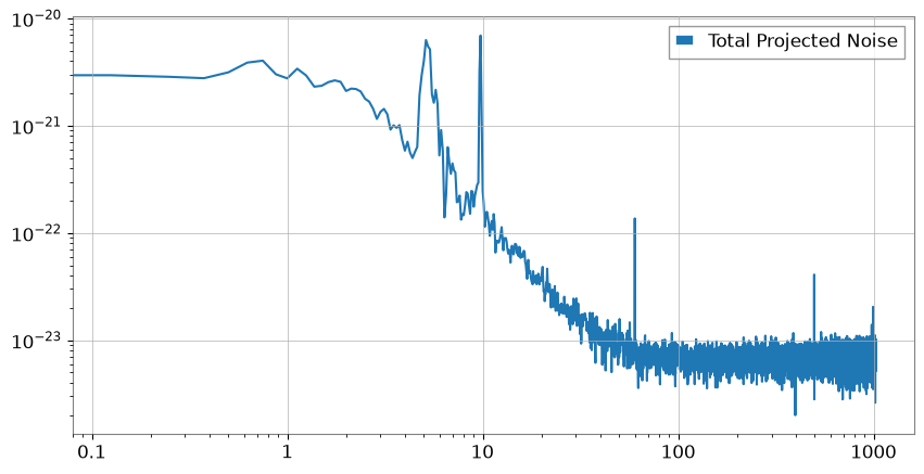
ノイズ投影 (Noise Projection): 伝達関数を用いて、補助チャンネルのノイズをメインチャンネルの単位に変換(投影)します。
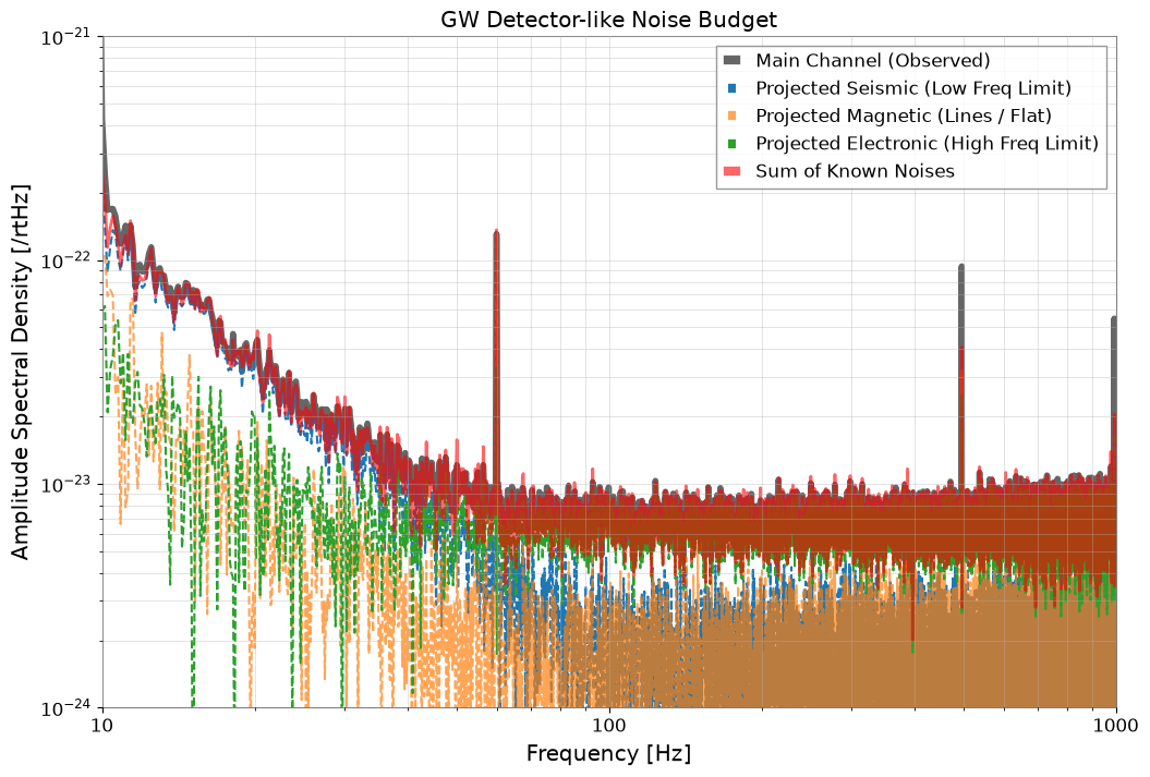
ノイズ予算の可視化 (Noise Budget Plot): すべてのノイズ源を重ね合わせ、観測された「U字型」スペクトルの内訳を明らかにします。
import matplotlib.pyplot as plt
import numpy as np
from scipy import signal

from gwexpy import TimeSeries, TimeSeriesDict
from gwexpy.noise.asd import from_pygwinc
from gwexpy.noise.wave import from_asd
1. 多チャンネルデータのシミュレーション (U字型スペクトルの作成)#
重力波検出器を模した感度曲線を作成します。
MAIN: 観測対象。低域で地面振動、高域でアクチュエータ/回路系のノイズが支配的な「下に凸」のスペクトルを持ちます。AUX_SEIS: 低周波の地面振動をモニター。AUX_MAG: 磁場モニター(60Hzの電源ラインを含む)。AUX_ELEC: 高周波側のノイズ源(例:制御システムや読み出し回路のノイズ)。
fs = 2048.0
duration = 64.0
t = np.arange(0, duration, 1 / fs)
n_samples = len(t)

np.random.seed(42)
rng = np.random.default_rng(42)

# Use an aLIGO-like ASD as the baseline target so the synthetic main channel resembles a detector sensitivity curve.
fmax = fs / 2
asd_main = from_pygwinc(
    "aLIGO", fmin=5.0, fmax=fmax, df=1.0 / duration, quantity="strain"
)
main_base = from_asd(asd_main, duration, fs, t0=0, rng=rng).highpass(5)

# --- Build auxiliary witness channels that stand in for candidate physical noise sources. ---
# 1. Ground motion dominates the low-frequency end, as seismic coupling often does in real detectors.
b_low, a_low = signal.butter(2, 2.0, fs=fs, btype="low")
seis_val = signal.lfilter(b_low, a_low, np.random.normal(0, 50.0, n_samples))
seis = TimeSeries(seis_val, sample_rate=fs, name="Seismic", unit="um")

# 2. Magnetic pickup contributes line features around mains harmonics plus a flatter broadband term.
mag_val = np.random.normal(0, 0.1, n_samples)
mag_val += 0.8 * np.sin(2 * np.pi * 60 * t)  # 60Hz
mag = TimeSeries(mag_val, sample_rate=fs, name="Magnetic", unit="nT")

# 3. Electronic noise becomes important at high frequency where the mechanical channels stop dominating.
elec_val = np.random.normal(0, 1.0, n_samples)
elec = TimeSeries(elec_val, sample_rate=fs, name="Electronic", unit="V")

# --- Mix those witnesses into the main channel so the observed strain-like spectrum is a sum of several physical contributions. ---
main = (
    main_base
    + seis * (2e-21 * main_base.unit / seis.unit)
    + mag * (1e-22 * main_base.unit / mag.unit)
    + elec * (2e-22 * main_base.unit / elec.unit)
)


# Keep the target and witness channels together so coherence and projection can be computed consistently.
tsd = TimeSeriesDict()
tsd["MAIN"] = main
tsd["AUX_SEIS"] = seis
tsd["AUX_MAG"] = mag
tsd["AUX_ELEC"] = elec

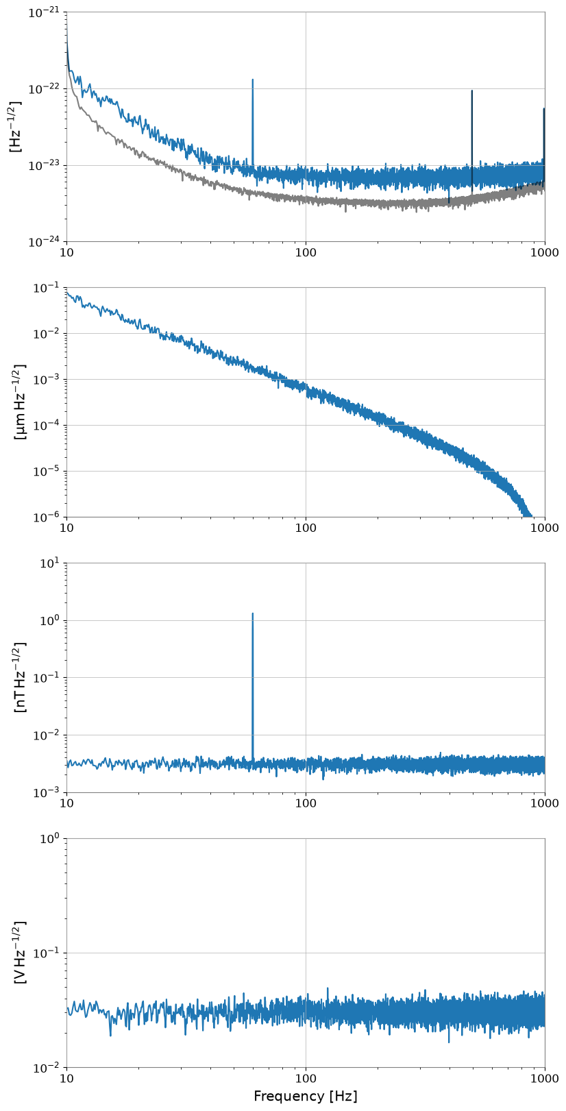
# Inspect the ASD first to confirm the synthetic main channel has the expected U-shaped detector-like profile.
asd_dict = tsd.asd(fftlength=8, overlap=4, method="welch")
plot = asd_dict.plot(xscale="log", yscale="log", subplots=True, sharex=True)
axes = plot.get_axes()
axes[0].plot(
    main_base.asd(fftlength=8, overlap=4, method="welch"), alpha=0.5, color="black"
)
axes[0].set_xlim(10, 1000)
axes[0].set_ylim(1e-24, 1e-21)
axes[1].set_ylim(1e-6, 1e-1)
axes[2].set_ylim(1e-3, 1e1)
axes[3].set_ylim(1e-2, 1e0)
plt.show()

# The MAIN channel now falls at low frequency and rises again at high frequency, which is the qualitative signature of different noise families dominating in different bands.
2. 相関解析 (Coherence Mapping)#
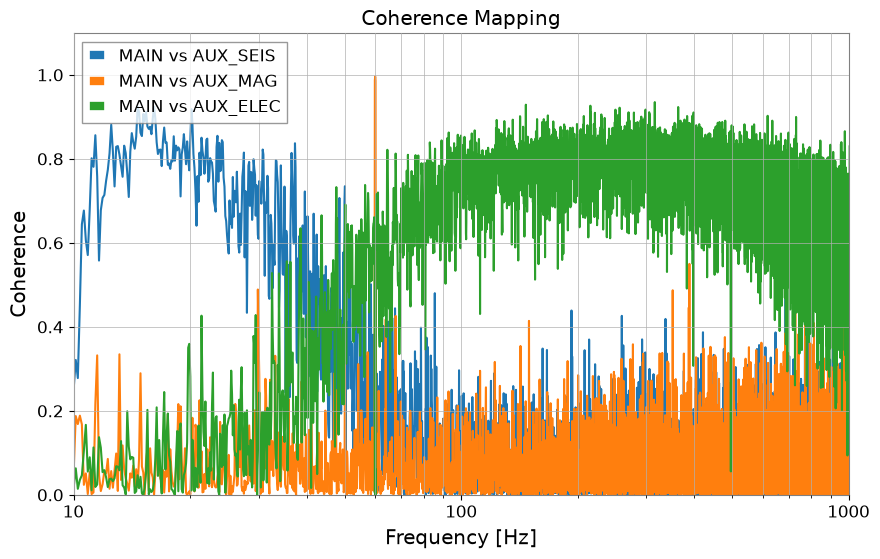
メインチャンネルの「U字」の左側、底、右側で、それぞれどのセンサーと高いコヒーレンスを持っているかを確認します。
aux_names = ["AUX_SEIS", "AUX_MAG", "AUX_ELEC"]

plt.figure(figsize=(10, 6))
for name in aux_names:
    coh = tsd["MAIN"].coherence(tsd[name], fftlength=8)
    plt.semilogx(coh.frequencies, coh.value, label=f"MAIN vs {name}")

plt.title("Coherence Mapping")
plt.xlabel("Frequency [Hz]")
plt.ylabel("Coherence")
plt.xlim(10, 1000)
plt.ylim(0, 1.1)
plt.legend()
plt.grid(True, which="both")
plt.show()

# Coherence shows which witness can explain the main channel in each band, but it still indicates shared structure rather than proof of causality.
3. 結合関数の推定#
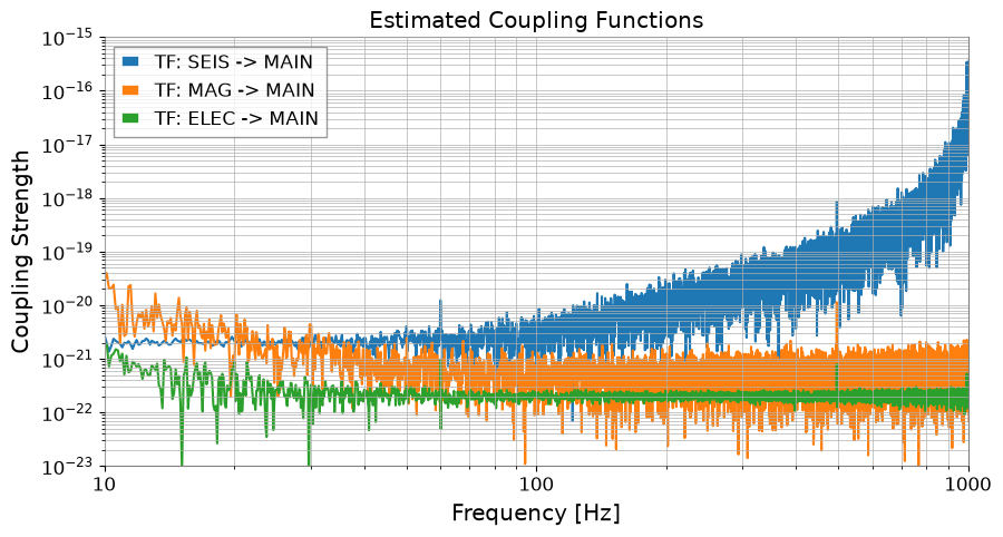
各帯域における漏れ込み係数(伝達関数)を推定します。
witness.transfer_function(MAIN) は、各チャンネルの値を使って出力と入力の数値的な比を推定します。GWpy と互換の結果は無次元です。補助チャンネルの ASD を掛ける前に MAIN.unit / witness.unit を明示的に付与することで、推定した各寄与の単位が MAIN の振幅単位/√Hz になります。伝達関数の推定と ASD には、同じ区間長、オーバーラップ、Hann 窓を使います。
二乗和平方根による合成は、ノイズ源の独立性を仮定します。補助チャンネル間で共通するノイズは重複して数えられる場合があります。また、有限長のデータからの推定値が、すべての周波数ビンで観測 ASD を下回るとは限りません。相関のある補助チャンネルを扱う場合は、Wiener フィルタのケーススタディを参照してください。
tf_seis = tsd["AUX_SEIS"].transfer_function(tsd["MAIN"], fftlength=8, overlap=4, window="hann")
tf_mag = tsd["AUX_MAG"].transfer_function(tsd["MAIN"], fftlength=8, overlap=4, window="hann")
tf_elec = tsd["AUX_ELEC"].transfer_function(tsd["MAIN"], fftlength=8, overlap=4, window="hann")

# GWpy-compatible transfer_function returns the numerical ratio without units.
# The ratio maps native witness values to native MAIN values, so attach MAIN/witness units.
tf_seis = tf_seis * (tsd["MAIN"].unit / tsd["AUX_SEIS"].unit)
tf_mag = tf_mag * (tsd["MAIN"].unit / tsd["AUX_MAG"].unit)
tf_elec = tf_elec * (tsd["MAIN"].unit / tsd["AUX_ELEC"].unit)

plt.figure(figsize=(10, 5))
plt.loglog(tf_seis.abs(), label="TF: SEIS -> MAIN")
plt.loglog(tf_mag.abs(), label="TF: MAG -> MAIN")
plt.loglog(tf_elec.abs(), label="TF: ELEC -> MAIN")

plt.xlim(10, 1000)
plt.ylim(1e-23, 1e-15)
plt.title("Estimated Coupling Functions")
plt.xlabel("Frequency [Hz]")
plt.ylabel("Coupling Strength")
plt.legend()
plt.grid(True, which="both")
plt.show()
4. ノイズ投影 (Noise Projection)#
main_ch = tsd["MAIN"]
proj_seis = asd_dict["AUX_SEIS"] * tf_seis.abs()
proj_mag = asd_dict["AUX_MAG"] * tf_mag.abs()
proj_elec = asd_dict["AUX_ELEC"] * tf_elec.abs()

# Sum the projected components in quadrature because approximately independent noise families add in power, not linearly in amplitude.
total_proj = (proj_seis**2 + proj_mag**2 + proj_elec**2) ** 0.5

# Plot the combined projection to compare the explained budget against the observed main spectrum.
plt.figure(figsize=(10, 5))
plt.loglog(total_proj, label="Total Projected Noise")
plt.legend()
plt.show()

# Every projection is now in MAIN amplitude / sqrt(Hz).
for projected in (proj_seis, proj_mag, proj_elec, total_proj):
    assert projected.unit.is_equivalent(asd_dict["MAIN"].unit)
    assert np.all(np.isfinite(projected.value))
    np.testing.assert_allclose(projected.frequencies.value, asd_dict["MAIN"].frequencies.value)
5. ノイズ予算の可視化 (Noise Budget Plot)#
「下に凸」のメインチャンネルのノイズが、どのように解説・分解されるかを表示します。
plt.figure(figsize=(12, 8))

# Plot the observed main ASD as the reference sensitivity curve we are trying to explain.
plt.loglog(
    asd_dict["MAIN"],
    label="Main Channel (Observed)",
    color="black",
    linewidth=4,
    alpha=0.6,
)

# Overlay each projected witness contribution to see which physical source dominates each band.
plt.loglog(proj_seis, label="Projected Seismic (Low Freq Limit)", ls="--")
plt.loglog(proj_mag, label="Projected Magnetic (Lines / Flat)", ls="--", alpha=0.7)
plt.loglog(proj_elec, label="Projected Electronic (High Freq Limit)", ls="--")

# The total projection is the hypothesis for the explained portion of the measured sensitivity.
plt.loglog(total_proj, label="Sum of Known Noises", color="red", linewidth=2, alpha=0.6)

plt.title("GW Detector-like Noise Budget")
plt.xlabel("Frequency [Hz]")
plt.ylabel(f"Amplitude Spectral Density [{main_ch.unit}/rtHz]")
plt.xlim(10, 1000)
plt.ylim(1e-24, 1e-21)
plt.legend(frameon=True, facecolor="white", loc="upper right")
plt.grid(True, which="both", ls="-", alpha=0.5)
plt.show()

# When the summed projection follows the measured curve, the budget supports the story that different noise mechanisms dominate different frequency ranges.