相互運用: 基本#
このノートブックでは、gwexpy の TimeSeries クラスに追加された新しい相互運用機能 (Interoperability Features) を紹介します。 gwexpy は、Pandas, Xarray, PyTorch, Astropy などの一般的なデータサイエンス・ライブラリとの間で、シームレスにデータを変換することができます。
gwexpy[all] はチュートリアル環境で使う宣言済み extra をまとめて導入しますが、すべての public interop backend を導入するものではありません。ROOT, torch, TensorFlow, JAX, PyCBC, Finesse などの個別 backend は、その bridge を使うときに直接導入してください。
目次#
汎用データ形式とデータ基盤
1.1. NumPy [Original GWpy]
1.2. Pandas との連携 [Original GWpy]
1.3. Polars [GWexpy New]
1.4. Xarray との連携 [Original GWpy]
1.5. Dask との連携 [GWexpy New]
1.6. JSON / Python Dict (to_json) (to_json) [GWexpy New]
データベースとストレージ層
2.1. HDF5 [Original GWpy]
2.2. SQLite [GWexpy New]
2.3. Zarr [GWexpy New]
2.4. netCDF4 [GWexpy New]
計算機科学・機械学習・高速計算
3.1. PyTorch との連携 [GWexpy New]
3.2. CuPy (CUDA 加速) [GWexpy New]
3.3. TensorFlow との連携 [GWexpy New]
3.4. JAX との連携 [GWexpy New]
天文学と重力波物理
4.1. PyCBC / LAL [Original GWpy]
4.2. Astropy との連携 [Original GWpy]
4.3. Specutils との連携 [GWexpy New]
4.4. Pyspeckit との連携 [GWexpy New]
素粒子物理・高エネルギー物理
5.1. CERN ROOT との連携 [GWexpy New]
5.2. ROOT オブジェクトからの復元 (
from_root)
地球物理・地震学・電磁気
6.1. ObsPy [Original GWpy]
6.2. SimPEG との連携 [GWexpy New]
6.3. MTH5 / MTpy [GWexpy New]
音響・オーディオ解析
7.1. Librosa / Pydub [GWexpy New]
医療・生体信号解析
8.1. MNE-Python [GWexpy New]
8.2. Elephant / quantities との連携 [GWexpy New]
8.3. Neo [GWexpy New]
まとめ
import warnings


import os

os.environ.setdefault("TF_CPP_MIN_LOG_LEVEL", "3")
'3'
import warnings

with warnings.catch_warnings():

    import matplotlib.pyplot as plt
    import numpy as np
    from astropy import units as u
    from gwpy.time import LIGOTimeGPS

    from gwexpy.timeseries import TimeSeries
/home/runner/micromamba/envs/gwexpy/lib/python3.11/site-packages/gwpy/time/_ligotimegps.py:42: UserWarning: Wswiglal-redir-stdio:

SWIGLAL standard output/error redirection is enabled in IPython.
This may lead to performance penalties. To disable locally, use:

with lal.no_swig_redirect_standard_output_error():
    ...

To disable globally, use:

lal.swig_redirect_standard_output_error(False)

Note however that this will likely lead to error messages from
LAL functions being either misdirected or lost when called from
Jupyter notebooks.

To suppress this warning, use:

import warnings
warnings.filterwarnings("ignore", "Wswiglal-redir-stdio")
import lal

  from lal import LIGOTimeGPS
# Create sample data
# Generate a 10-second, 100Hz sine wave
rate = 100 * u.Hz
dt = 1 / rate
t0 = LIGOTimeGPS(1234567890, 0)
duration = 10 * u.s
size = int(rate * duration)
times = np.arange(size) * dt.value
data = np.sin(2 * np.pi * 1.0 * times)  # 1Hz sine wave

ts = TimeSeries(data, t0=t0, dt=dt, unit="V", name="demo_signal")
print("Original TimeSeries:")
print(ts)
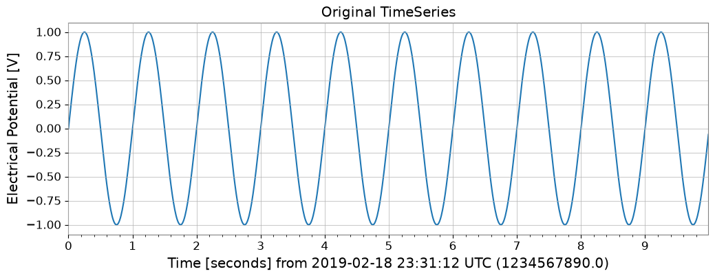
ts.plot(title="Original TimeSeries");
Original TimeSeries:
TimeSeries([ 0.        ,  0.06279052,  0.12533323, ...,
            -0.18738131, -0.12533323, -0.06279052],
           unit: V,
           t0: 1234567890.0 1 / Hz,
           dt: 0.01 1 / Hz,
           name: demo_signal,
           channel: None)
1. 汎用データ形式・データ基盤#
1.1. NumPy [Original GWpy]#
NumPy:NumPy は Python における数値計算の基盤ライブラリで、多次元配列と高速な数学演算を提供します。📚 NumPy ドキュメント
TimeSeries.value や np.asarray(ts) で NumPy 配列を取得できます。
1.2. Pandas との連携 [Original GWpy]#
Pandas:Pandas はデータ分析と操作のための強力なライブラリで、DataFrame と Series による柔軟なデータ構造を提供します。📚 Pandas ドキュメント
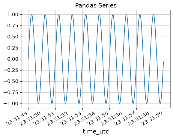
to_pandas() メソッドを使うと、TimeSeries を pandas.Series に変換できます。 インデックスは datetime (UTC), gps, seconds (Unix timestamp) から選択可能です。
try:
    # Convert to Pandas Series (default is datetime index)
    s_pd = ts.to_pandas(index="datetime")
    print("\n--- Converted to Pandas Series ---")
    display(s_pd)
    fig, ax = plt.subplots()
    s_pd.plot(ax=ax, title="Pandas Series")
    plt.show()
    plt.close(fig)

    # Restore TimeSeries from Pandas Series
    ts_restored = TimeSeries.from_pandas(s_pd, unit="V")
    print("\n--- Restored TimeSeries from Pandas ---")
    print(ts_restored)

    del s_pd, ts_restored

except ImportError:
    print("Pandas is not installed.")
--- Converted to Pandas Series ---
time_utc
2019-02-18 23:31:49+00:00           0.000000
2019-02-18 23:31:49.010000+00:00    0.062791
2019-02-18 23:31:49.020000+00:00    0.125333
2019-02-18 23:31:49.030000+00:00    0.187381
2019-02-18 23:31:49.040000+00:00    0.248690
                                      ...
2019-02-18 23:31:58.949991+00:00   -0.309017
2019-02-18 23:31:58.959991+00:00   -0.248690
2019-02-18 23:31:58.969990+00:00   -0.187381
2019-02-18 23:31:58.979990+00:00   -0.125333
2019-02-18 23:31:58.989990+00:00   -0.062791
Name: demo_signal, Length: 1000, dtype: float64
--- Restored TimeSeries from Pandas ---
TimeSeries([ 0.        ,  0.06279052,  0.12533323, ...,
            -0.18738131, -0.12533323, -0.06279052],
           unit: V,
           t0: 1234567927.0 s,
           dt: 0.009999990463256836 s,
           name: demo_signal,
           channel: None)
1.3. Polars [GWexpy New]#
Polars:Polars は Rust で実装された高性能な DataFrame ライブラリで、大規模データ処理に優れます。📚 Polars ドキュメント
to_polars() で Polars DataFrame/Series に変換できます。
try:
    import polars as pl

    _ = pl
    # TimeSeries -> Polars DataFrame
    df_pl = ts.to_polars()
    print("--- Polars DataFrame ---")
    print(df_pl.head())

    # Plot using Polars/Matplotlib
    plt.figure()
    data_col = [c for c in df_pl.columns if c != "time"][0]
    plt.plot(df_pl["time"], df_pl[data_col])
    plt.title("Polars Data Plot")
    plt.show()

    # Recover to TimeSeries
    from gwexpy.timeseries import TimeSeries

    ts_recovered = TimeSeries.from_polars(df_pl)
    print("Recovered from Polars:", ts_recovered)

    del df_pl, ts_recovered

except ImportError:
    print("Polars not installed.")
Polars not installed.
1.4. Xarray との連携 [Original GWpy]#
xarray:xarray は多次元ラベル付き配列のためのライブラリで、NetCDF データの操作や気象・地球科学データの解析に広く使われます。📚 xarray ドキュメント
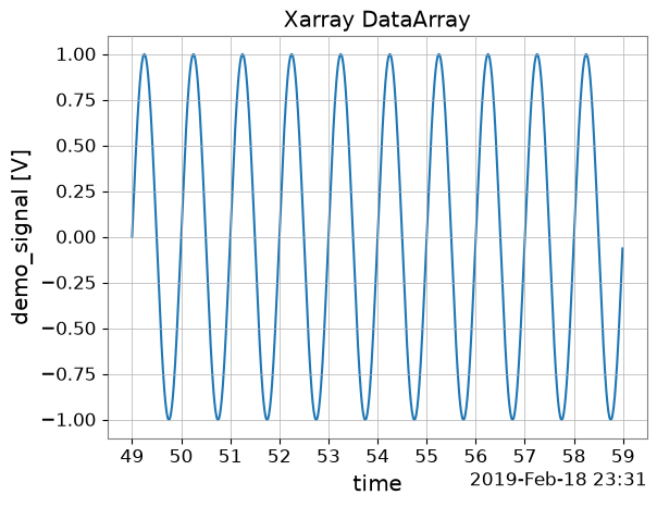
xarray は多次元のラベル付き配列を扱う強力なライブラリです。to_xarray() でメタデータを保持したまま変換できます。
try:
    # Convert to Xarray DataArray
    da = ts.to_xarray()
    print("\n--- Converted to Xarray DataArray ---")
    print(da)
    # Verify metadata (attrs) is preserved
    print("Attributes:", da.attrs)

    da.plot()
    plt.title("Xarray DataArray")
    plt.show()
    plt.close()

    # Restore
    ts_x = TimeSeries.from_xarray(da)
    print("\n--- Restored TimeSeries from Xarray ---")
    print(ts_x)

    del da, ts_x

except ImportError:
    print("Xarray is not installed.")
--- Converted to Xarray DataArray ---
<xarray.DataArray 'demo_signal' (time: 1000)> Size: 8kB
array([ 0.        ,  0.06279052,  0.12533323, ..., -0.18738131,
       -0.12533323, -0.06279052], shape=(1000,))
Coordinates:
  * time     (time) datetime64[us] 8kB 2019-02-18T23:31:49 ... 2019-02-18T23:...
Attributes:
    unit:        V
    epoch:       1234567890.0
    time_coord:  datetime
    name:        demo_signal
Attributes: {'unit': 'V', 'epoch': 1234567890.0, 'time_coord': 'datetime', 'name': 'demo_signal'}
--- Restored TimeSeries from Xarray ---
TimeSeries([ 0.        ,  0.06279052,  0.12533323, ...,
            -0.18738131, -0.12533323, -0.06279052],
           unit: V,
           t0: 1234567927.0 s,
           dt: 0.009999990463256836 s,
           name: demo_signal,
           channel: None)
1.5. Dask との連携 [GWexpy New]#
Dask:Dask は並列計算のためのライブラリで、NumPy/Pandas を超える大規模データの処理を可能にします。📚 Dask ドキュメント
try:
    import dask.array as da

    _ = da
    # Convert to Dask Array
    dask_arr = ts.to_dask(chunks="auto")
    print("\n--- Converted to Dask Array ---")
    print(dask_arr)

    # Restore (compute=True loads immediately)
    ts_from_dask = TimeSeries.from_dask(dask_arr, t0=ts.t0, dt=ts.dt, unit=ts.unit)
    print("Recovered from Dask:", ts_from_dask)

    del dask_arr, ts_from_dask

except ImportError:
    print("Dask not installed.")
--- Converted to Dask Array ---
dask.array<array, shape=(1000,), dtype=float64, chunksize=(1000,), chunktype=numpy.ndarray>
Recovered from Dask: TimeSeries([ 0.        ,  0.06279052,  0.12533323, ...,
            -0.18738131, -0.12533323, -0.06279052],
           unit: V,
           t0: 1234567890.0 1 / Hz,
           dt: 0.01 1 / Hz,
           name: None,
           channel: None)
1.6. JSON / Python Dict (to_json) [GWexpy New]#
JSON:JSON(JavaScript Object Notation)は軽量なデータ交換形式で、Python 標準ライブラリでサポートされています。📚 JSON ドキュメント
to_json() や to_dict() で JSON 互換の辞書形式を出力できます。
import json

# TimeSeries -> JSON string
ts_json = ts.to_json()
print("--- JSON Representation (Partial) ---")
print(ts_json[:500] + "...")

# Plot data by loading back from JSON
ts_dict_temp = json.loads(ts_json)
plt.figure()
plt.plot(ts_dict_temp["data"])
plt.title("Plot from JSON Data")
plt.show()

# Recover from JSON
from gwexpy.timeseries import TimeSeries

ts_recovered = TimeSeries.from_json(ts_json)
print("Recovered from JSON:", ts_recovered)

del ts_json, ts_dict_temp, ts_recovered
--- JSON Representation (Partial) ---
{
  "t0": 1234567890.0,
  "dt": 0.01,
  "unit": "V",
  "name": "demo_signal",
  "channel": null,
  "data": [
    0.0,
    0.06279051952931337,
    0.12533323356430426,
    0.1873813145857246,
    0.2486898871648548,
    0.3090169943749474,
    0.3681245526846779,
    0.4257792915650727,
    0.4817536741017153,
    0.5358267949789967,
    0.5877852522924731,
    0.6374239897486896,
    0.6845471059286886,
    0.7289686274214116,
    0.7705132427757893,
    0.8090169943749475,
    0.84432792550201...
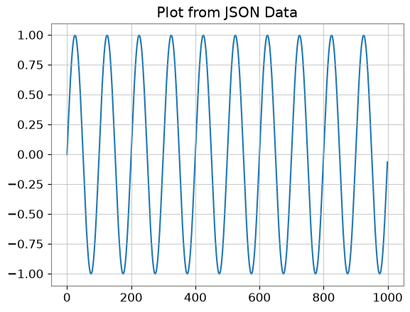
Recovered from JSON: TimeSeries([ 0.        ,  0.06279052,  0.12533323, ...,
            -0.18738131, -0.12533323, -0.06279052],
           unit: V,
           t0: 1234567890.0 s,
           dt: 0.01 s,
           name: demo_signal,
           channel: None)
2. データベース・ストレージ層#
2.1. HDF5 [Original GWpy]#
HDF5:HDF5 は大規模な科学データを効率的に保存・管理するための階層的データ形式です。Python からは h5py ライブラリ経由でアクセスできます。📚 HDF5 ドキュメント
to_hdf5_dataset() で HDF5 への保存をサポート。
try:
    import tempfile

    import h5py

    with tempfile.NamedTemporaryFile(suffix=".h5") as tmp:
        # TimeSeries -> HDF5
        with h5py.File(tmp.name, "w") as f:
            ts.to_hdf5_dataset(f, "dataset_01")

        # Read back and display
        with h5py.File(tmp.name, "r") as f:
            ds = f["dataset_01"]
            print("--- HDF5 Dataset Info ---")
            print(f"Shape: {ds.shape}, Dtype: {ds.dtype}")
            print("Attributes:", dict(ds.attrs))

            # Recover
            from gwexpy.timeseries import TimeSeries

            ts_recovered = TimeSeries.from_hdf5_dataset(f, "dataset_01")
            print("Recovered from HDF5:", ts_recovered)

            ts_recovered.plot()
            plt.title("Recovered from HDF5")
            plt.show()

            del ds, ts_recovered

except ImportError:
    print("h5py not installed.")
--- HDF5 Dataset Info ---
Shape: (1000,), Dtype: float64
Attributes: {'dt': np.float64(0.01), 'name': 'demo_signal', 't0': np.float64(1234567890.0), 'unit': 'V'}
Recovered from HDF5: TimeSeries([ 0.        ,  0.06279052,  0.12533323, ...,
            -0.18738131, -0.12533323, -0.06279052],
           unit: V,
           t0: 1234567890.0 s,
           dt: 0.01 s,
           name: demo_signal,
           channel: None)
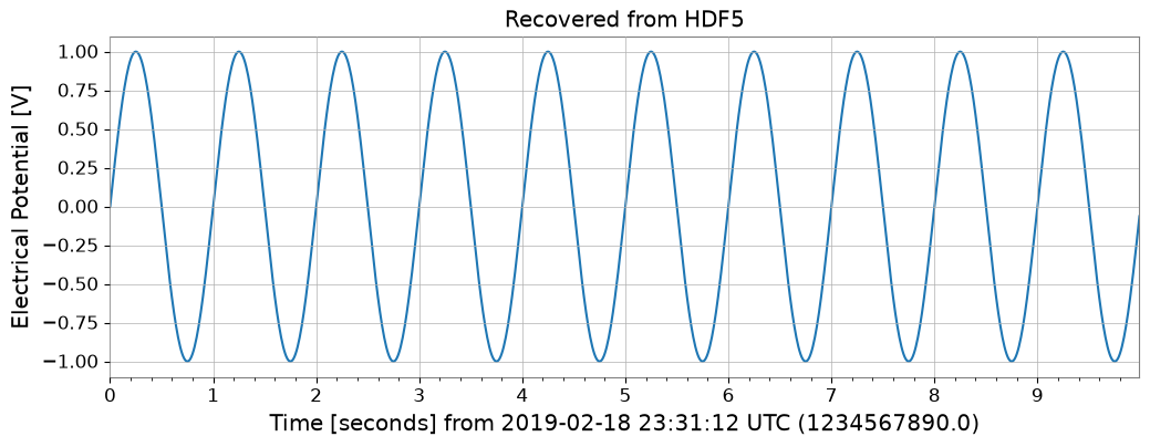
2.2. SQLite [GWexpy New]#
SQLite:SQLite は軽量な組み込み型 SQL データベースエンジンで、Python 標準ライブラリに含まれています。📚 SQLite ドキュメント
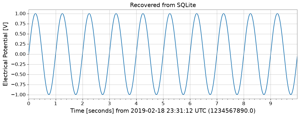
to_sqlite() で DB 永続化をサポート。
import sqlite3

conn = sqlite3.connect(":memory:")

# TimeSeries -> SQLite
series_id = ts.to_sqlite(conn, series_id="test_series")
print(f"Saved to SQLite with ID: {series_id}")

# Verify data in SQL
cursor = conn.cursor()
row = cursor.execute("SELECT * FROM series WHERE series_id=?", (series_id,)).fetchone()
print("Metadata from SQL:", row)

# Recover
from gwexpy.timeseries import TimeSeries

ts_recovered = TimeSeries.from_sqlite(conn, series_id)
print("Recovered from SQLite:", ts_recovered)

ts_recovered.plot()
plt.title("Recovered from SQLite")
plt.show()

del series_id, conn, cursor, ts_recovered
Saved to SQLite with ID: test_series
Metadata from SQL: ('test_series', '', 'V', 1234567890.0, 0.01, 1000, '{"name": "demo_signal"}')
Recovered from SQLite: TimeSeries([ 0.        ,  0.06279052,  0.12533323, ...,
            -0.18738131, -0.12533323, -0.06279052],
           unit: V,
           t0: 1234567890.0 s,
           dt: 0.01 s,
           name: test_series,
           channel: None)
2.3. Zarr [GWexpy New]#
Zarr:Zarr はチャンク化・圧縮された多次元配列のためのストレージ形式で、クラウドストレージとの統合に優れます。📚 Zarr ドキュメント
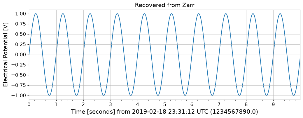
to_zarr() でクラウドストレージ向き形式に対応。
try:
    import os
    import tempfile

    import zarr

    with tempfile.TemporaryDirectory() as tmpdir:
        store_path = os.path.join(tmpdir, "test.zarr")
        # TimeSeries -> Zarr
        ts.to_zarr(store_path, path="timeseries")

        # Read back
        z = zarr.open(store_path, mode="r")
        ds = z["timeseries"]
        print("--- Zarr Array Info ---")
        print(ds.info)

        # Recover
        from gwexpy.timeseries import TimeSeries

        ts_recovered = TimeSeries.from_zarr(store_path, "timeseries")
        print("Recovered from Zarr:", ts_recovered)

        ts_recovered.plot()
        plt.title("Recovered from Zarr")
        plt.show()

        del z, ds, ts_recovered

except ImportError:
    print("zarr not installed.")
--- Zarr Array Info ---
Type               : Array
Zarr format        : 3
Data type          : Float64(endianness='little')
Fill value         : 0.0
Shape              : (1000,)
Chunk shape        : (1000,)
Order              : C
Read-only          : True
Store type         : LocalStore
Filters            : ()
Serializer         : BytesCodec(endian=<Endian.little: 'little'>)
Compressors        : (ZstdCodec(level=0, checksum=False),)
No. bytes          : 8000 (7.8K)
Recovered from Zarr: TimeSeries([ 0.        ,  0.06279052,  0.12533323, ...,
            -0.18738131, -0.12533323, -0.06279052],
           unit: V,
           t0: 1234567890.0 s,
           dt: 0.01 s,
           name: demo_signal,
           channel: None)
2.4. netCDF4 [GWexpy New]#
netCDF4:netCDF4 は気象・海洋・地球科学データの標準形式で、自己記述的なデータ構造を持ちます。📚 netCDF4 ドキュメント
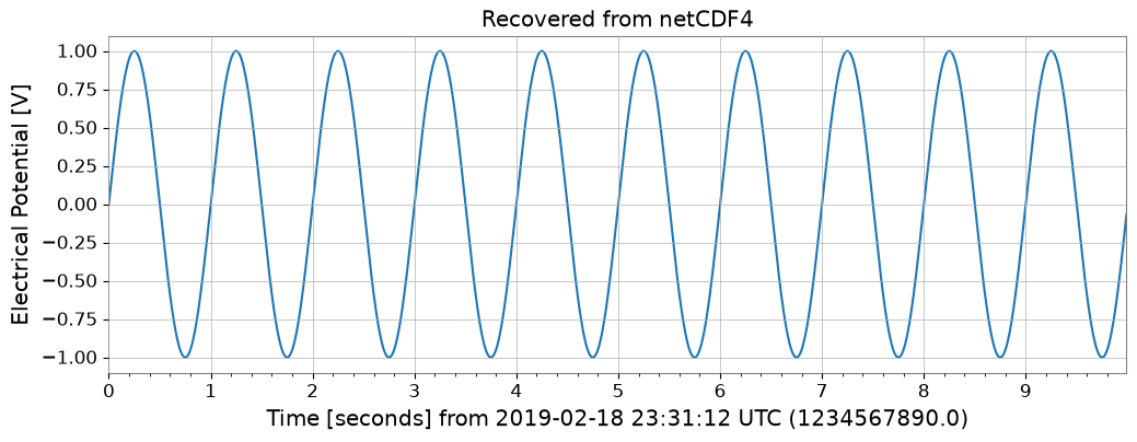
to_netcdf4() で気象・海洋データの標準に対応。
try:
    import tempfile
    from pathlib import Path

    import netCDF4

    with tempfile.TemporaryDirectory() as tmpdir:
        path = Path(tmpdir) / "gwexpy_timeseries.nc"

        # TimeSeries -> netCDF4
        with netCDF4.Dataset(path, "w", format="NETCDF3_CLASSIC") as ds:
            ts.to_netcdf4(ds, "my_signal")

        # Read back
        with netCDF4.Dataset(path, "r") as ds:
            v = ds.variables["my_signal"]
            print("--- netCDF4 Variable Info ---")
            print(v)

            # Recover
            from gwexpy.timeseries import TimeSeries

            ts_recovered = TimeSeries.from_netcdf4(ds, "my_signal")
            print("Recovered from netCDF4:", ts_recovered)

            ts_recovered.plot()
            plt.title("Recovered from netCDF4")
            plt.show()

            del v, ts_recovered

except ImportError:
    print("netCDF4 not installed.")
<frozen importlib._bootstrap>:241: RuntimeWarning: numpy.ndarray size changed, may indicate binary incompatibility. Expected 16 from C header, got 96 from PyObject
--- netCDF4 Variable Info ---
<class 'netCDF4.Variable'>
float64 my_signal(time)
    t0: 1234567890.0
    dt: 0.01
    units: V
    long_name: demo_signal
unlimited dimensions:
current shape = (1000,)
filling on, default _FillValue of 9.969209968386869e+36 used
Recovered from netCDF4: TimeSeries([ 0.        ,  0.06279052,  0.12533323, ...,
            -0.18738131, -0.12533323, -0.06279052],
           unit: V,
           t0: 1234567890.0 s,
           dt: 0.01 s,
           name: demo_signal,
           channel: None)
3. 情報科学・機械学習・加速計算#
3.1. PyTorch との連携 [GWexpy New]#
PyTorch:PyTorch は動的計算グラフと GPU 高速化をサポートするディープラーニングフレームワークです。📚 PyTorch ドキュメント
ディープラーニングの前処理として、TimeSeries を直接 torch.Tensor に変換できます。GPU転送も可能です。
import os

os.environ.setdefault("TF_CPP_MIN_LOG_LEVEL", "3")

try:
    import torch

    # Convert to PyTorch Tensor
    tensor = ts.to_torch(dtype=torch.float32)
    print("\n--- Converted to PyTorch Tensor ---")
    print(f"Tensor shape: {tensor.shape}, dtype: {tensor.dtype}")

    # Restore from Tensor (t0, dt must be specified separately)
    ts_torch = TimeSeries.from_torch(tensor, t0=ts.t0, dt=ts.dt, unit="V")
    print("\n--- Restored from Torch ---")
    print(ts_torch)

    del tensor, ts_torch

except ImportError:
    print("PyTorch is not installed.")
PyTorch is not installed.
3.2. CuPy (CUDA 加速) [GWexpy New]#
CuPy:CuPy は NumPy 互換の GPU 配列ライブラリで、NVIDIA CUDA を用いた高速計算を可能にします。📚 CuPy ドキュメント
GPU 上での計算を可能にする CuPy 配列へ変換できます。
from gwexpy.interop import is_cupy_available

if is_cupy_available():
    import cupy as cp

    # TimeSeries -> CuPy
    y_gpu = ts.to_cupy()
    print("--- CuPy Array (on GPU) ---")
    print(y_gpu)

    # Simple processing on GPU
    y_gpu_filt = y_gpu * 2.0

    # Plot (must move to CPU for plotting)
    plt.figure()
    plt.plot(cp.asnumpy(y_gpu_filt))
    plt.title("CuPy Data (Moved to CPU for plot)")
    plt.show()

    # Recover
    from gwexpy.timeseries import TimeSeries

    ts_recovered = TimeSeries.from_cupy(y_gpu_filt, t0=ts.t0, dt=ts.dt)
    print("Recovered from CuPy:", ts_recovered)

    del y_gpu, y_gpu_filt, ts_recovered

else:
    print("CuPy or CUDA driver not available.")
CuPy or CUDA driver not available.
3.3. TensorFlow との連携 [GWexpy New]#
TensorFlow:TensorFlow は Google が開発した機械学習プラットフォームで、大規模な本番環境に優れます。📚 TensorFlow ドキュメント
import warnings

with warnings.catch_warnings():

    try:
        import os

        os.environ.setdefault("TF_CPP_MIN_LOG_LEVEL", "3")
        warnings.filterwarnings("ignore", category=UserWarning, module=r"google\.protobuf\..*")
        warnings.filterwarnings("ignore", category=UserWarning, message=r"Protobuf gencode version.*")
        import tensorflow as tf

        _ = tf
        # Convert to TensorFlow Tensor
        tf_tensor = ts.to_tensorflow()
        print("\n--- Converted to TensorFlow Tensor ---")
        print(f"Tensor shape: {tf_tensor.shape}")
        print(f"Tensor dtype: {tf_tensor.dtype}")

        # Restore
        ts_from_tensorflow = TimeSeries.from_tensorflow(
            tf_tensor, t0=ts.t0, dt=ts.dt, unit=ts.unit
        )
        print("Recovered from TF:", ts_from_tensorflow)

        del tf_tensor, ts_from_tensorflow

    except ImportError:
        pass
3.4. JAX との連携 [GWexpy New]#
JAX:JAX は Google が開発した高性能な数値計算ライブラリで、自動微分と XLA コンパイルによる高速化を特徴とします。📚 JAX ドキュメント
try:
    import os

    os.environ["XLA_PYTHON_CLIENT_PREALLOCATE"] = "false"
    import jax

    _ = jax
    import jax.numpy as jnp

    _ = jnp
    # Convert to JAX Array
    jax_arr = ts.to_jax()
    print("\n--- Converted to JAX Array ---")
    print(f"Array shape: {jax_arr.shape}")

    # Restore
    ts_from_jax = TimeSeries.from_jax(jax_arr, t0=ts.t0, dt=ts.dt, unit=ts.unit)
    print("Recovered from JAX:", ts_from_jax)

    del jax_arr, ts_from_jax
except ImportError:
    print("JAX not installed.")
JAX not installed.
4. 天文学・重力波物理学#
4.1. PyCBC / LAL [Original GWpy]#
LAL:LAL(LIGO Algorithm Library)は LIGO/Virgo の公式解析ライブラリで、重力波解析の基盤を提供します。📚 LAL ドキュメント
PyCBC:PyCBC は重力波データ解析のためのライブラリで、信号探索やパラメータ推定に使われます。📚 PyCBC ドキュメント
重力波解析の標準ツールとの互換性を備えています。
4.2. Astropy との連携 [Original GWpy]#
Astropy:Astropy は天文学のための Python ライブラリで、座標変換、時系変換、単位系などをサポートします。📚 Astropy ドキュメント
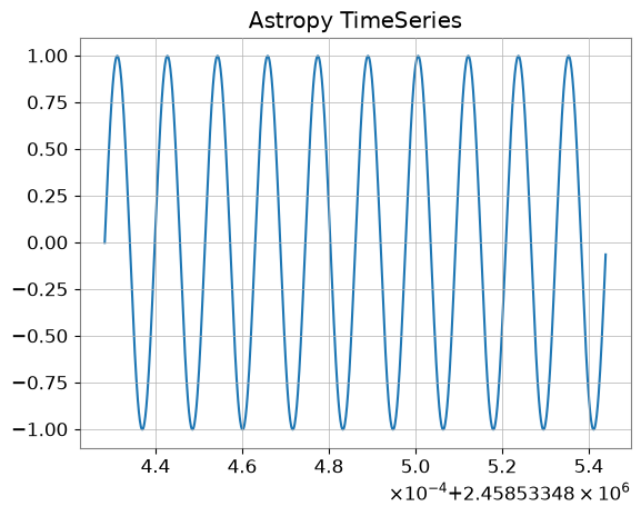
天文学分野で標準的な astropy.timeseries.TimeSeries との相互変換もサポートしています。
try:
    # Convert to Astropy TimeSeries
    ap_ts = ts.to_astropy_timeseries()
    print("\n--- Converted to Astropy TimeSeries ---")
    print(ap_ts[:5])
    fig, ax = plt.subplots()
    ax.plot(ap_ts.time.jd, ap_ts["value"])
    plt.title("Astropy TimeSeries")
    plt.show()
    plt.close()

    # Restore
    ts_astro = TimeSeries.from_astropy_timeseries(ap_ts)
    print("\n--- Restored from Astropy ---")
    print(ts_astro)

    del ap_ts, ts_astro

except ImportError:
    print("Astropy is not installed.")
--- Converted to Astropy TimeSeries ---
     time            value
------------- -------------------
 1234567890.0                 0.0
1234567890.01 0.06279051952931337
1234567890.02 0.12533323356430426
1234567890.03  0.1873813145857246
1234567890.04  0.2486898871648548
--- Restored from Astropy ---
TimeSeries([ 0.        ,  0.06279052,  0.12533323, ...,
            -0.18738131, -0.12533323, -0.06279052],
           unit: dimensionless,
           t0: 1234567890.0 s,
           dt: 0.009999990463256836 s,
           name: None,
           channel: None)
4.3. Specutils との連携 [GWexpy New]#
specutils:specutils は天文スペクトルデータの操作と解析のための Astropy 関連パッケージです。📚 specutils ドキュメント
FrequencySeries は、Astropy エコシステムのスペクトル解析ライブラリ specutils の Spectrum1D オブジェクトと相互変換可能です。 単位 (Units) や周波数軸が適切に保持されます。
try:
    import specutils

    _ = specutils

    from gwexpy.frequencyseries import FrequencySeries

    # FrequencySeries -> specutils.Spectrum1D
    fs = FrequencySeries(
        np.random.random(100), frequencies=np.linspace(10, 100, 100), unit="Jy"
    )
    spec = fs.to_specutils()
    print("specutils Spectrum1D:", spec)
    print("Spectral axis unit:", spec.spectral_axis.unit)

    # specutils.Spectrum1D -> FrequencySeries
    fs_rec = FrequencySeries.from_specutils(spec)
    print("Restored FrequencySeries unit:", fs_rec.unit)

    del fs, spec, fs_rec

except ImportError:
    print("specutils library not found. Skipping example.")
specutils library not found. Skipping example.
4.4. Pyspeckit との連携 [GWexpy New]#
PySpecKit:PySpecKit は電波天文学のためのスペクトル解析ツールキットで、スペクトル線フィッティングなどをサポートします。📚 PySpecKit ドキュメント
FrequencySeries は、汎用的なスペクトル解析ツールキット pyspeckit の Spectrum オブジェクトとも連携可能です。
try:
    import pyspeckit

    _ = pyspeckit
    from gwexpy.frequencyseries import FrequencySeries

    # FrequencySeries -> pyspeckit.Spectrum
    fs = FrequencySeries(np.random.random(100), frequencies=np.linspace(10, 100, 100))
    spec = fs.to_pyspeckit()
    print("pyspeckit Spectrum length:", len(spec.data))

    # pyspeckit.Spectrum -> FrequencySeries
    fs_rec = FrequencySeries.from_pyspeckit(spec)
    print("Restored FrequencySeries length:", len(fs_rec))

    del fs, spec, fs_rec

except ImportError:
    print("pyspeckit library not found. Skipping example.")
pyspeckit library not found. Skipping example.
5. 素粒子物理学・高エネルギー物理#
5.1. CERN ROOT との連携 [GWexpy New]#
ROOT:ROOT は CERN が開発した高エネルギー物理のためのデータ解析フレームワークです。📚 ROOT ドキュメント
高エネルギー物理学で標準的なツールである ROOT との相互運用が強化されました。 gwexpy の Series オブジェクトを ROOT の TGraph や TH1D, TH2D に高速に変換したり、ROOT ファイルを作成することができます。 逆に、ROOT オブジェクトから TimeSeries などを復元することも可能です。
Note: この機能を使用するには ROOT (PyROOT) がインストールされている必要があります。
try:
    import numpy as np
    import ROOT

    from gwexpy.timeseries import TimeSeries

    # Prepare data
    t = np.linspace(0, 10, 1000)
    data = np.sin(2 * np.pi * 1.0 * t) + np.random.normal(0, 0.5, size=len(t))
    ts = TimeSeries(data, dt=t[1] - t[0], name="signal")

    # --- 1. Convert to TGraph ---
    # Vectorized high-speed conversion
    graph = ts.to_tgraph()

    # Plot on ROOT canvas
    c1 = ROOT.TCanvas("c1", "TGraph Example", 800, 600)
    graph.SetTitle("ROOT TGraph;GPS Time [s];Amplitude")
    graph.Draw("AL")
    c1.Draw()
    # c1.SaveAs("signal_graph.png") # To save as an image

    print(f"Created TGraph: {graph.GetName()} with {graph.GetN()} points")

    # --- 2. Convert to TH1D (Histogram) ---
    # Convert as histogram (binning is automatic or can be specified)
    hist = ts.to_th1d()

    c2 = ROOT.TCanvas("c2", "TH1D Example", 800, 600)
    hist.SetTitle("ROOT TH1D;GPS Time [s];Amplitude")
    hist.SetLineColor(ROOT.kRed)
    hist.Draw()
    c2.Draw()

    print(f"Created TH1D: {hist.GetName()} with {hist.GetNbinsX()} bins")

    del t, data, graph, hist, c1, c2

except ImportError as e:
    print(f"An error occurred: {e}")
An error occurred: No module named 'ROOT'
5.2. ROOT オブジェクトからの復元 (from_root)#
ROOT:ROOT は CERN が開発した高エネルギー物理のためのデータ解析フレームワークです。📚 ROOT ドキュメント
既存の ROOT ファイルにあるヒストグラムやグラフを読み込んで、解析しやすい gwexpy オブジェクトに戻すことができます。
from gwexpy.interop import from_root

try:
    if "hist" in locals() and hist:
        # ROOT TH1D -> TimeSeries
        # Reads histogram bin contents as time series data
        ts_restored = from_root(TimeSeries, hist)

        print(f"Restored TimeSeries: {ts_restored.name}")
        print(ts_restored)

        # Restore from TGraph similarly
        ts_from_graph = from_root(TimeSeries, graph)
        print(f"Restored from TGraph: {len(ts_from_graph)} samples")

        del ts_restored, ts_from_graph

except ImportError:
    pass  # ROOT (PyROOT) is not installed
6. 地球物理学・地震学・電磁気学#
6.1. ObsPy [Original GWpy]#
ObsPy:ObsPy は地震学データの取得・処理・解析のための Python ライブラリで、MiniSEED などの形式をサポートします。📚 ObsPy ドキュメント
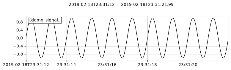
地震学で標準的な ObsPy との相互運用をサポート。
try:
    import obspy

    _ = obspy
    # TimeSeries -> ObsPy Trace
    tr = ts.to_obspy()
    print("--- ObsPy Trace ---")
    print(tr)

    # Plot using ObsPy
    tr.plot()

    # Recover to TimeSeries
    from gwexpy.timeseries import TimeSeries

    ts_recovered = TimeSeries.from_obspy(tr)
    print("Recovered from ObsPy:", ts_recovered)

    del tr, ts_recovered

except ImportError:
    print("ObsPy not installed.")
--- ObsPy Trace ---
.demo_signal.. | 2019-02-18T23:31:12.000000Z - 2019-02-18T23:31:21.990000Z | 100.0 Hz, 1000 samples
Recovered from ObsPy: TimeSeries([ 0.        ,  0.06279052,  0.12533323, ...,
            -0.18738131, -0.12533323, -0.06279052],
           unit: dimensionless,
           t0: 1234567890.0 s,
           dt: 0.01 s,
           name: .demo_signal..,
           channel: None)
try:
    import obspy

    _ = obspy
    tr = ts.to_obspy()
    print("ObsPy Trace:", tr)

    del tr

except ImportError:
    print("ObsPy not installed.")
ObsPy Trace: .demo_signal.. | 2019-02-18T23:31:12.000000Z - 2019-02-18T23:31:21.990000Z | 100.0 Hz, 1000 samples
6.2. SimPEG との連携 [GWexpy New]#
SimPEG:SimPEG は地球物理の逆問題のためのシミュレーション・推定フレームワークです。📚 SimPEG ドキュメント
gwexpy は、地球物理学のフォワード計算・反転モデリングライブラリである SimPEG との連携をサポートしています。 TimeSeries (TDEM) および FrequencySeries (FDEM) を simpeg.data.Data オブジェクトに変換したり、その逆を行ったりできます。
try:
    import numpy as np
    import simpeg

    _ = simpeg
    from simpeg import maps

    _ = maps

    from gwexpy.frequencyseries import FrequencySeries
    from gwexpy.timeseries import TimeSeries

    # --- TimeSeries -> SimPEG (TDEM assumption) ---
    ts = TimeSeries(np.random.normal(size=100), dt=0.01, unit="A/m^2")
    simpeg_data_td = ts.to_simpeg(location=np.array([0, 0, 0]))
    print("SimPEG TDEM data shape:", simpeg_data_td.dobs.shape)

    # --- FrequencySeries -> SimPEG (FDEM assumption) ---
    fs = FrequencySeries(
        np.random.normal(size=10) + 1j * 0.1, frequencies=np.logspace(0, 3, 10)
    )
    simpeg_data_fd = fs.to_simpeg(location=np.array([0, 0, 0]), orientation="z")
    print("SimPEG FDEM data shape:", simpeg_data_fd.dobs.shape)

    del simpeg_data_td, simpeg_data_fd, fs

except ImportError:
    print("SimPEG library not found. Skipping example.")
SimPEG library not found. Skipping example.
6.3. MTH5 / MTpy [GWexpy New]#
MTH5:MTH5 は地磁気地電流(MT)データのための HDF5 ベースのデータ形式です。📚 MTH5 ドキュメント
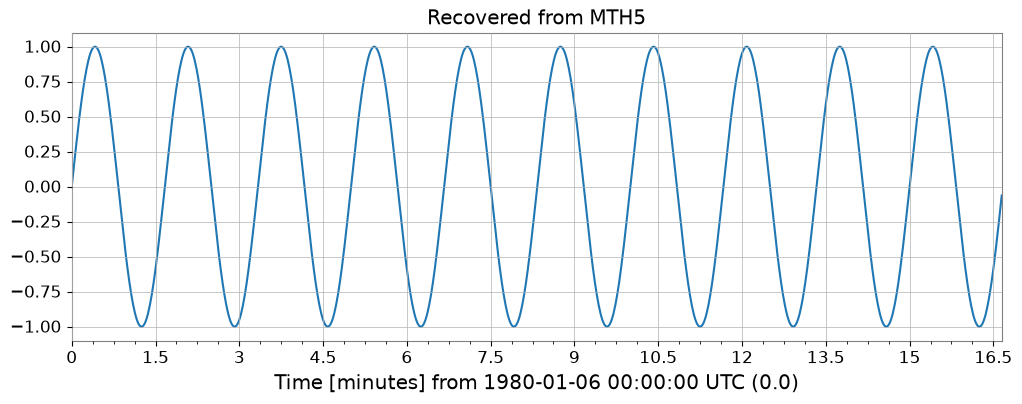
地磁気地電流法データの MTH5 保存に対応。
try:
    import logging
    import tempfile

    logging.getLogger("mth5").setLevel(logging.ERROR)
    logging.getLogger("mt_metadata").setLevel(logging.ERROR)

    import mth5

    _ = mth5
    with tempfile.NamedTemporaryFile(suffix=".h5") as tmp:
        from gwexpy.interop.mt_ import from_mth5, to_mth5

        # TimeSeries -> MTH5
        # We need to provide station and run names for MTH5 structure
        to_mth5(ts, tmp.name, station="SITE01", run="RUN01")
        print("Saved to temporary MTH5 file")

        # Display structure info if needed, or just recover
        # Recover
        ts_recovered = from_mth5(tmp.name, "SITE01", "RUN01", ts.name or "Ex")
        print("Recovered from MTH5:", ts_recovered)

        ts_recovered.plot()
        plt.title("Recovered from MTH5")
        plt.show()

        del ts_recovered

except ImportError:
    print("mth5 not installed.")
2026-09-06T10:32:35.499042+0000 | INFO | mth5.mth5 | _initialize_file | line: 900 | Initialized MTH5 0.2.0 file /tmp/tmpljpg984c.h5 in mode a
2026-09-06T10:32:36.252499+0000 | INFO | mth5.mth5 | close_mth5 | line: 1035 | Flushing and closing /tmp/tmpljpg984c.h5
Saved to temporary MTH5 file
2026-09-06T10:32:36.476819+0000 | INFO | mth5.mth5 | close_mth5 | line: 1035 | Flushing and closing /tmp/tmpljpg984c.h5
Recovered from MTH5: TimeSeries([ 0.        ,  0.06279052,  0.12533323, ...,
            -0.18738131, -0.12533323, -0.06279052],
           unit: dimensionless,
           t0: 0.0 s,
           dt: 1.0 s,
           name: demo_signal,
           channel: None)
7. 音響・音声解析#
7.1. Librosa / Pydub [GWexpy New]#
pydub:pydub は音声ファイルの操作(編集・変換・エフェクト)のためのシンプルなライブラリです。📚 pydub ドキュメント
librosa:librosa は音声・音楽解析のためのライブラリで、スペクトル解析やビート検出などの機能を提供します。📚 librosa ドキュメント
音声処理ライブラリ Librosa や Pydub との連携をサポート。
try:
    import librosa

    _ = librosa
    import matplotlib.pyplot as plt

    # TimeSeries -> Librosa (y, sr)
    y, sr = ts.to_librosa()
    print(f"--- Librosa Data ---\nSignal shape: {y.shape}, Sample rate: {sr}")

    # Plot using librosa style (matplotlib)
    plt.figure()
    plt.plot(y[:1000])  # Plot first 1000 samples
    plt.title("Librosa Audio Signal (Zoom)")
    plt.show()

    # Recover to TimeSeries
    from gwexpy.timeseries import TimeSeries

    ts_recovered = TimeSeries(y, dt=1.0 / sr)
    print("Recovered from Librosa:", ts_recovered)

    del y, sr
except ImportError:
    print("Librosa not installed.")
Librosa not installed.
8. 医学・生体信号解析#
8.1. MNE-Python [GWexpy New]#
MNE:MNE-Python は EEG・MEG データ解析のためのライブラリで、神経科学研究で広く使われます。📚 MNE ドキュメント
脳電図 (EEG/MEG) 解析パッケージ MNE との連携。
try:
    import mne

    _ = mne
    # TimeSeries -> MNE Raw
    raw = ts.to_mne()
    print("--- MNE Raw ---")
    print(raw)

    # Display info
    print(raw.info)

    # Recover to TimeSeries
    from gwexpy.timeseries import TimeSeries

    ts_recovered = TimeSeries.from_mne(raw, channel=ts.name or "ch0")
    print("Recovered from MNE:", ts_recovered)

    del raw, ts_recovered

except ImportError:
    print("MNE not installed.")
MNE not installed.
try:
    import mne

    _ = mne
    raw = ts.to_mne()
    print("MNE Raw:", raw)

    del raw
except ImportError:
    print("MNE not installed.")
MNE not installed.
8.2. Elephant / quantities との連携 [GWexpy New]#
gwexpy の FrequencySeries や Spectrogram は、quantities.Quantity オブジェクトと相互変換可能です。 これは Elephant や Neo との連携に役立ちます。
※ 事前に pip install quantities が必要です。
try:
    import numpy as np
    import quantities as pq

    _ = pq
    from gwexpy.frequencyseries import FrequencySeries

    # Create FrequencySeries
    freqs = np.linspace(0, 100, 101)
    data_fs = np.random.random(101)
    fs = FrequencySeries(data_fs, frequencies=freqs, unit="V")

    # to_quantities
    q_obj = fs.to_quantities(units="mV")
    print("Quantities object:", q_obj)

    # from_quantities
    fs_new = FrequencySeries.from_quantities(q_obj, frequencies=freqs)
    print("Restored FrequencySeries unit:", fs_new.unit)

    del freqs, data_fs, fs, q_obj, fs_new

except ImportError:
    print("quantities library not found. Skipping example.")
quantities library not found. Skipping example.
8.3. Neo [GWexpy New]#
Neo:Neo は電気生理学データ(神経科学)のためのデータ構造ライブラリで、さまざまな形式への入出力をサポートします。📚 Neo ドキュメント
電気生理データの共通規格 Neo への変換をサポート。
try:
    import neo

    _ = neo
    # TimeSeries -> Neo AnalogSignal
    # to_neo is available in gwexpy.interop
    # Note: TimeseriesMatrix is preferred for multi-channel Neo conversion,
    # but we can convert single TimeSeries by wrapping it.
    from gwexpy.interop import from_neo, to_neo

    _ = from_neo
    _ = to_neo
    # For single TimeSeries, we might need a Matrix wrapper or direct helper.
    # Assuming helper exists or using Matrix:
    from gwexpy.timeseries import TimeSeriesMatrix

    tm = TimeSeriesMatrix(
        ts.value[None, None, :], t0=ts.t0, dt=ts.dt, channel_names=[ts.name]
    )
    sig = tm.to_neo()

    print("--- Neo AnalogSignal ---")
    print(sig)

    # Display/Plot
    plt.figure()
    plt.plot(sig.times, sig)
    plt.title("Neo AnalogSignal Plot")
    plt.show()

    # Recover
    tm_recovered = TimeSeriesMatrix.from_neo(sig)
    ts_recovered = tm_recovered[0]
    print("Recovered from Neo:", ts_recovered)

    del tm, tm_recovered, sig, ts_recovered

except ImportError:
    print("neo not installed.")
neo not installed.
9. 音響・電磁シミュレーション連携(追加ライブラリ)#
以下のセクションでは、室内音響シミュレーション・電磁場シミュレーション・非構造格子メッシュデータ・マルチテーパースペクトル推定の4つの追加連携モジュールを扱います。
9.1. Pyroomacoustics — 室内インパルス応答(RIR)#
pyroomacoustics は室内音響をシミュレートし、室内インパルス応答(RIR)を提供します。
room.rirはrir[mic_index][source_index]という規約に従います(外側のインデックス = マイク)。
try:
    from unittest.mock import MagicMock

    import numpy as np


    TimeSeries = MagicMock()
    TimeSeries.__name__ = "TimeSeries"

    # Mock room: 2 mics x 2 sources — real layout: rir[mic][source]
    room = MagicMock()
    room.fs = 16000
    rir_data = [
        [np.array([1.0, 0.5, 0.2, 0.0]), np.array([0.8, 0.4, 0.1, 0.0])],  # mic 0
        [np.array([0.9, 0.3, 0.1, 0.0]), np.array([0.7, 0.2, 0.05, 0.0])], # mic 1
    ]
    room.rir = rir_data

    # from_pyroomacoustics_rir(cls, room, source=0, mic=0) -> TimeSeries
    # Returns rir[mic=0][source=0]
    print("from_pyroomacoustics_rir: source=0, mic=0 ->", rir_data[0][0])
    print("Tip: room.rir convention is rir[mic_index][source_index]")
except ImportError as e:
    print(f"Skipped (pyroomacoustics not installed or mock error): {e}")
from_pyroomacoustics_rir: source=0, mic=0 -> [1.  0.5 0.2 0. ]
Tip: room.rir convention is rir[mic_index][source_index]
9.2. OpenEMS — HDF5 電磁場ダンプ#
openEMS は場のデータを HDF5 に書き出します。データセットが
"Time"(TD)または"frequency"(FD)属性を持つ場合、axis0 には物理値が使われます。そうでない場合は、整数インデックスがフォールバックとして使われます。
try:
    import os
    import tempfile

    import h5py
    import numpy as np

    from gwexpy.fields import VectorField
    from gwexpy.interop.openems_ import from_openems_hdf5

    # Create a minimal openEMS-style HDF5 file with Time attributes
    with tempfile.NamedTemporaryFile(suffix=".h5", delete=False) as tmp:
        tmp_path = tmp.name

    with h5py.File(tmp_path, "w") as h5:
        mesh = h5.create_group("Mesh")
        mesh.create_dataset("x", data=np.linspace(0, 1, 4))
        mesh.create_dataset("y", data=np.linspace(0, 1, 4))
        mesh.create_dataset("z", data=np.linspace(0, 1, 4))

        td = h5.create_group("FieldData/TD")
        for i, t in enumerate([1e-9, 2e-9, 3e-9]):
            ds = td.create_dataset(f"step_{i}", data=np.ones((4, 4, 4, 3)))
            ds.attrs["Time"] = t  # physical time in seconds

    vf = from_openems_hdf5(VectorField, tmp_path, dump_type=0)
    print(f"VectorField axes: {vf['x'].shape}, axis0={list(vf['x']._axis0_index)}")
    print("axis0 contains physical time values (1e-9, 2e-9, 3e-9 s)")
    os.unlink(tmp_path)
except ImportError as e:
    print(f"Skipped: {e}")
VectorField axes: (3, 4, 4, 4), axis0=[<Quantity 1.e-09>, <Quantity 2.e-09>, <Quantity 3.e-09>]
axis0 contains physical time values (1e-9, 2e-9, 3e-9 s)
9.3. Meshio — 非構造格子メッシュ → ScalarField#
meshio は 40 以上のメッシュ形式(VTK、XDMF、Gmsh、…)を読み込みます。補間でサポートされるのは
point_dataのみです。cell_dataしかない場合はValueErrorが送出されます — 先にpoint_dataに変換してください。
try:
    from unittest.mock import MagicMock

    import numpy as np

    from gwexpy.fields import ScalarField
    from gwexpy.interop.meshio_ import from_meshio

    # 2D triangular mesh with scalar temperature field
    nx, ny = 15, 15
    x = np.linspace(0, 1, nx)
    y = np.linspace(0, 1, ny)
    xx, yy = np.meshgrid(x, y)
    pts = np.column_stack([xx.ravel(), yy.ravel(), np.zeros(nx * ny)])

    mesh = MagicMock()
    mesh.points = pts
    mesh.point_data = {"temperature": pts[:, 0] ** 2 + pts[:, 1] ** 2}
    mesh.cell_data = {}
    mesh.cells = []

    sf = from_meshio(ScalarField, mesh, grid_resolution=0.1)
    print(f"ScalarField shape: {sf.shape}  (axis0, nx, ny, 1)")
    print(f"Value at centre ≈ {float(np.asarray(sf.value)[0, sf.shape[1]//2, sf.shape[2]//2, 0]):.3f}")
except ImportError as e:
    print(f"Skipped: {e}")
ScalarField shape: (1, 11, 11, 1)  (axis0, nx, ny, 1)
Value at centre ≈ 0.500
9.4. マルチテーパースペクトル推定#
2 つの multitaper パッケージがサポートされます:
from_mtspec経由の multitaper(Prieto)と、from_mtspec_array経由の mtspec(Krischer)です。常にプレーンなスペクトルを得るにはcls=FrequencySeriesを、利用可能なら信頼区間を含めるにはcls=FrequencySeriesDictを渡します。
try:
    from unittest.mock import MagicMock

    import numpy as np

    # Simulate FrequencySeries / FrequencySeriesDict via mock registry
    class _FS(list):
        def __init__(self, data, *, frequencies, name="", unit=None):
            super().__init__(data)
            self.frequencies = frequencies
            self.name = name

    class _FSD(dict):
        pass

    from gwexpy.interop._registry import ConverterRegistry
    ConverterRegistry.register_constructor("FrequencySeries", _FS)
    ConverterRegistry.register_constructor("FrequencySeriesDict", _FSD)

    from gwexpy.interop.multitaper_ import from_mtspec

    # Mock MTSpec object with CI
    n = 100
    freq = np.linspace(0, 50, n)
    mt = MagicMock()
    mt.freq = freq
    mt.spec = np.abs(np.random.default_rng(0).standard_normal(n)) + 0.1
    mt.spec_ci = np.column_stack([mt.spec * 0.8, mt.spec * 1.2])

    # cls=_FS -> always FrequencySeries (CI discarded)
    result_fs = from_mtspec(_FS, mt, include_ci=True)
    print(f"cls=FrequencySeries -> type: {type(result_fs).__name__}")

    # cls=_FSD -> FrequencySeriesDict with CI keys
    result_fsd = from_mtspec(_FSD, mt, include_ci=True)
    print(f"cls=FrequencySeriesDict -> type: {type(result_fsd).__name__}, keys: {list(result_fsd.keys())}")
except ImportError as e:
    print(f"Skipped: {e}")
cls=FrequencySeries -> type: _FS
cls=FrequencySeriesDict -> type: _FSD, keys: ['psd', 'ci_lower', 'ci_upper']
/tmp/ipykernel_5050/297830298.py:17: UserWarning: ConverterRegistry: overwriting constructor 'FrequencySeries' (<class 'gwexpy.frequencyseries.frequencyseries.FrequencySeries'> -> <class '__main__._FS'>)
  ConverterRegistry.register_constructor("FrequencySeries", _FS)
/tmp/ipykernel_5050/297830298.py:18: UserWarning: ConverterRegistry: overwriting constructor 'FrequencySeriesDict' (<class 'gwexpy.frequencyseries.collections.FrequencySeriesDict'> -> <class '__main__._FSD'>)
  ConverterRegistry.register_constructor("FrequencySeriesDict", _FSD)
よくある落とし穴と解釈上の注意#
すべての変換が可逆だと思い込むこと: 多くの bridge は配列本体を渡せても、単位、
t0、dt、チャネル名、軸ラベルまでは自動で完全保存されない場合があります。direct I/O と interop を混同すること:
to_*()/from_*()はオブジェクト変換の説明であり、Class.read(..., format=...)やobj.write(...)と同じ保存保証を意味しません。時刻情報やサンプルレートが曖昧なまま解釈すること: 変換自体が成功しても、タイムゾーンやサンプリング情報が十分に運ばれていないと、整列や比較の解釈を誤ります。
規約を確認せずに数値だけ比較すること: FFT 正規化、周波数刻み、軸順序、shape の約束はライブラリごとに異なることがあり、見た目が似ていても意味は一致しない場合があります。
一部対応を全面対応だと読むこと: ここで動く例は、特定のクラスや経路での実例であり、すべての round-trip や補助属性まで保証するものではありません。
図が似ているだけで意味も同じだと判断すること: プロットが近く見えても、単位、座標、インデックスの意味が変わっている可能性があります。図だけでなく metadata を確認してください。
10. まとめ#
gwexpy は多種多様な bilimti 向けライブラリとの相互運用を提供し、既存のエコシステムとのシームレスな統合を可能にします。