ウィーナーフィルタ: コヒーレント雑音の差し引き#
複数の witness センサーが 同じ物理ノイズ源を重なって見ている とき、各 witness を独立に引くと二重差し引きが起きることがあります。
この notebook は legacy の MIMO 例を公開 docs 向けに整理し、多入力ウィーナーフィルタ行列の物理的意味に絞っています。
import matplotlib.pyplot as plt
import numpy as np
from scipy import signal

from gwexpy import FrequencySeriesDict, TimeSeries, TimeSeriesDict
from gwexpy.noise.asd import from_pygwinc
from gwexpy.noise.wave import from_asd

fs = 2048.0
duration = 64.0
t = np.arange(0, duration, 1 / fs)
n = len(t)
np.random.seed(123)
rng = np.random.default_rng(123)

# Two independent physical sources are mixed into two witnesses with different weights, creating crosstalk between sensors.
b_low, a_low = signal.butter(2, 5.0, fs=fs, btype="low")
s1 = signal.lfilter(b_low, a_low, np.random.normal(0, 10.0, n))
b_band, a_band = signal.iirpeak(120.0, 30.0, fs=fs)
s2 = signal.lfilter(b_band, a_band, np.random.normal(0, 2.0, n)) + np.random.normal(0, 0.1, n)
aux1_val = 1.0 * s1 + 0.4 * s2 + np.random.normal(0, 0.05, n)
aux2_val = 0.6 * s1 + 1.0 * s2 + np.random.normal(0, 0.05, n)

asd_main = from_pygwinc("aLIGO", fmin=5.0, fmax=fs / 2, df=1.0 / duration, quantity="strain")
tsd = TimeSeriesDict()
tsd["MAIN"] = from_asd(asd_main, duration, fs, t0=0, rng=rng).highpass(5.0)
tsd["AUX1"] = TimeSeries(aux1_val, sample_rate=fs, unit="V")
tsd["AUX2"] = TimeSeries(aux2_val, sample_rate=fs, unit="V")

# Add witness-coupled noise into MAIN so subtraction has a coherent target to remove.
tsd["MAIN"] += tsd["AUX1"] / tsd["AUX1"].unit * tsd["MAIN"].unit * 2e-22
tsd["MAIN"] += tsd["AUX2"] / tsd["AUX2"].unit * tsd["MAIN"].unit * 5e-22
1. 相互相関行列を推定する#
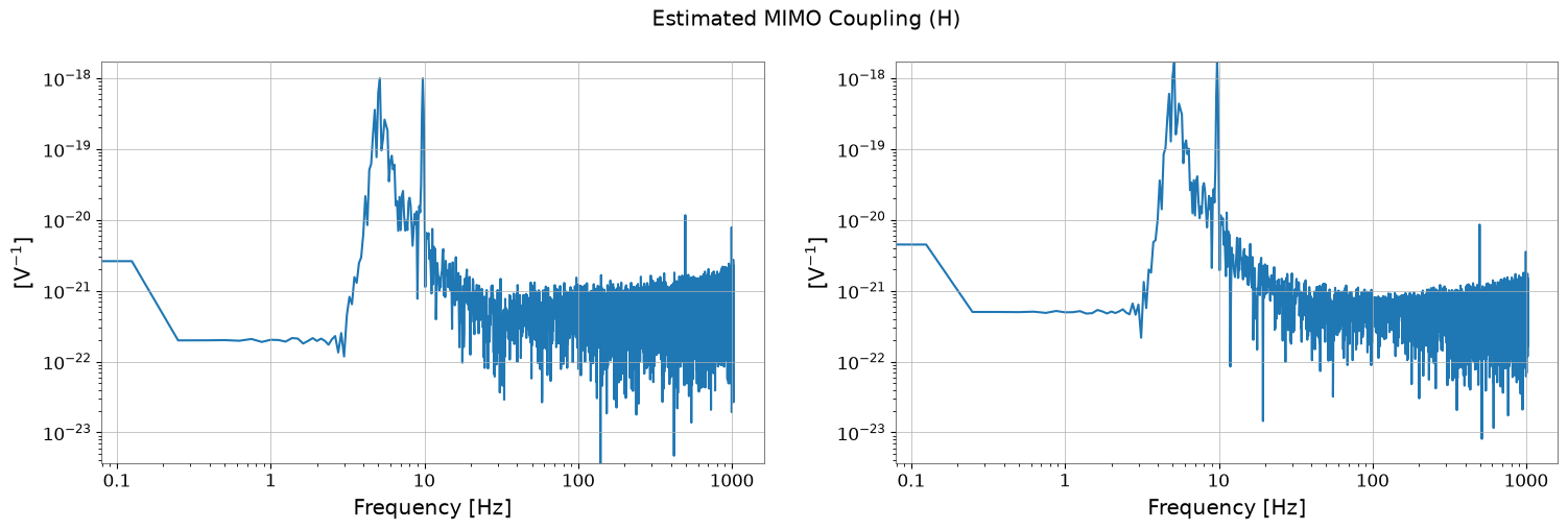
重要なのは witness 同士が独立ではないことです。Cxx が witness 間相関、Cyx が target と witness の相関を表します。
この例では \(C_{ij}=\langle X_i^*X_j\rangle\) という規約を使うため、補助チャンネルから MAIN への変換を表す行ベクトルのフィルタは \(H=(C_{yx}C_{xx}^{-1})^*\) となります。行列のすべての要素に同一の Hann 窓、オーバーラップ、算術平均を使います。継承したスペクトルのメタデータは異なるチャンネル間の単位を推論しないため、数値的な伝達関数の推定値に MAIN/補助チャンネルの単位を明示的に付与します。
FFT と逆 FFT は既存の正規化を使用し、サンプルレートによる補正や係数 2 の追加補正は行いません。この合成例の補助チャンネル行列は非特異です。冗長な測定補助チャンネルに適用する場合は、条件数を確認し、根拠のある正則化を選択してください。
aux_names = ["AUX1", "AUX2"]
aux_tsd = TimeSeriesDict({k: tsd[k] for k in aux_names})

# Use the same mean averaging for diagonal PSDs and off-diagonal CSDs.
spectral_options = dict(fftlength=8.0, overlap=4.0, window="hann", average="mean")
cxx = aux_tsd.csd_matrix(**spectral_options)
cyx = TimeSeriesDict({"MAIN": tsd["MAIN"]}).csd_matrix(
    other=aux_tsd, **spectral_options
)

# Cij = <conj(X_i) X_j>; conjugate to map witnesses to MAIN.
H_lowres = (cyx @ cxx.inv()).conj()
# Attach the physical output/input units to the numerical transfer estimates.
for j, name in enumerate(aux_names):
    H_lowres.meta[0, j].unit = tsd["MAIN"].unit / tsd[name].unit
    assert np.all(np.isfinite(H_lowres[0, j].value))
H_lowres.abs().plot(xscale="log", yscale="log").suptitle("Estimated MIMO Coupling (H)")
plt.show()
2. 予測して差し引く#
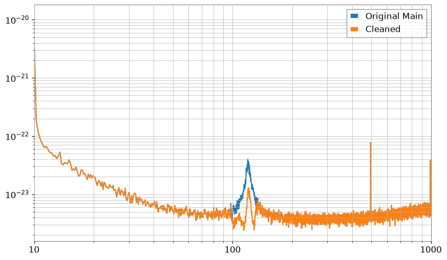
差し引くべきなのは witness で再構成できるコヒーレント成分だけであり、target 固有の不可避雑音は残るはずです。
tsd_fft = tsd.fft()
H = H_lowres.interpolate(tsd_fft["MAIN"].frequencies)
X_mat = FrequencySeriesDict({k: tsd_fft[k] for k in aux_names}).to_matrix()

# Projection estimates the part of MAIN that can be reconstructed from the witnesses.
Y_proj = (H @ X_mat)[0, 0]
projected_ts = Y_proj.ifft()
assert projected_ts.unit == tsd["MAIN"].unit
assert projected_ts.dt == tsd["MAIN"].dt
assert projected_ts.t0 == tsd["MAIN"].t0
assert projected_ts.size == tsd["MAIN"].size
cleaned_ts = tsd["MAIN"] - projected_ts.bandpass(100, 130).real

asd_raw = tsd["MAIN"].asd(fftlength=4.0)
asd_cleaned = cleaned_ts.asd(fftlength=4.0)

plt.figure(figsize=(10, 6))
plt.loglog(asd_raw, label="Original Main")
plt.loglog(asd_cleaned, label="Cleaned")
plt.xlim(10, 1000)
plt.legend()
plt.grid(True, which="both")
plt.show()